Warm-start QAOA con el addon de Qiskit Optimization Mapper

Estimación de uso: 9 minutos en un Heron r3 (NOTA: Esto es solo una estimación. Tu tiempo de ejecución puede variar.)

Resultados de aprendizaje

• Cómo mapear un problema de max-cut a una formulación cuántica de Optimización Binaria Cuadrática No Restringida (QUBO) usando qiskit-addon-opt-mapper

• Cómo implementar y ejecutar QAOA estándar en un simulador

• Cómo aplicar WS-QAOA calculando la relajación del programa cuadrático (QP) y construyendo el circuito de warm-start

• Cómo comparar la convergencia de energía y la calidad de la solución entre QAOA estándar y WS-QAOA

Requisitos previos

• Tutorial de QAOA

• Tutorial avanzado de QAOA

Contexto

El Algoritmo de Optimización Aproximada Cuántica (QAOA) es un algoritmo híbrido cuántico-clásico diseñado para resolver problemas de optimización combinatoria como max-cut y formulaciones generales de QUBO. Para una introducción fundamental a QAOA en Qiskit, consulta el tutorial de QAOA; para técnicas más avanzadas de construcción de circuitos, consulta el tutorial avanzado de QAOA.

En QAOA estándar:

• El estado inicial es la superposición uniforme $|+\rangle^{\otimes n}$.
• Los parámetros variacionales se inicializan aleatoriamente.
• Un optimizador clásico busca parámetros que minimicen la función de costo.

Sin embargo, para tamaños de problema prácticos y hardware cuántico ruidoso, la inicialización aleatoria puede llevar a una convergencia lenta, mínimos locales pobres, y un mayor costo de optimización.

Warm-start QAOA (WS-QAOA) mejora esto al incorporar conocimientos de optimización clásica directamente en el circuito cuántico. Este tutorial sigue los métodos introducidos por Egger, Mareček y Woerner en Warm-starting quantum optimization. La idea clave es:

1. Resolver una relajación continua del problema binario original (un programa cuadrático sobre $[0,1]^n$ en lugar de $\{0,1\}^n$).

2. Codificar la solución relajada $c^*_i \in [0,1]$ en un estado inicial personalizado usando ángulos de rotación $Y$, $\theta_i = 2\arcsin(\sqrt{c^*_i})$, de modo que el qubit $i$ comience en un estado cuya probabilidad de medir $|1\rangle$ sea $c^*_i$.

3. Reemplazar el mixer $X$ estándar con un mixer personalizado cuyo estado fundamental es el estado inicial de warm-start, asegurando que el algoritmo comience cerca de la solución clásica y pueda explorar el vecindario.

Un parámetro de regularización $\varepsilon \in [0, 0.5]$ recorta $c^*_i$ alejándolo de 0 y 1 para evitar problemas de alcanzabilidad; los qubits inicializados en $|0\rangle$ o $|1\rangle$ no pueden ser movidos por el Hamiltoniano de costo. En $\varepsilon = 0.5$, WS-QAOA se reduce exactamente a QAOA estándar.

El modelado del problema usa el paquete qiskit-addon-opt-mapper, cuya clase de aplicación Maxcut construye el QUBO directamente a partir de un grafo, y cuyos conversores y traductores mapean el problema resultante a Hamiltonianos cuánticos.

Requisitos

Antes de comenzar este tutorial, asegúrate de tener instalado lo siguiente:

• Qiskit SDK v2.0 o posterior, con soporte de visualización

• Qiskit Runtime v0.43 o posterior (pip install qiskit-ibm-runtime)

• Optimization Mapper Qiskit addon (pip install qiskit-addon-opt-mapper)

• SciPy (pip install scipy)

• NetworkX (pip install networkx)

Configuración

Importa todas las bibliotecas necesarias y define las funciones auxiliares usadas a lo largo de este tutorial.

# Added by doQumentation — required packages for this notebook
!pip install -q matplotlib networkx numpy qiskit qiskit-addon-opt-mapper qiskit-ibm-runtime scipy

import numpy as np
import matplotlib.pyplot as plt
import networkx as nx
from scipy.optimize import minimize

from qiskit.circuit import QuantumCircuit, ParameterVector
from qiskit.circuit.library import qaoa_ansatz
from qiskit.quantum_info import Statevector
from qiskit.primitives import StatevectorEstimator, StatevectorSampler
from qiskit.transpiler.preset_passmanagers import generate_preset_pass_manager
from qiskit_ibm_runtime import (
    QiskitRuntimeService,
    Session,
    EstimatorOptions,
    EstimatorV2 as Estimator,
    SamplerV2 as Sampler,
)

from qiskit_addon_opt_mapper.applications import Maxcut
from qiskit_addon_opt_mapper.converters import OptimizationProblemToQubo
from qiskit_addon_opt_mapper.translators import to_ising

Ejemplo de simulador a pequeña escala

Usamos un pequeño problema de max-cut en un grafo ponderado como nuestro ejemplo de referencia. Max-cut pregunta: dado un grafo $G=(V,E)$ con pesos de aristas $w_{ij}$, encuentra una partición de los vértices en dos conjuntos $S$ y $\bar{S}$ que maximice el peso total de las aristas que cruzan el corte.

Como problema de minimización QUBO, max-cut se puede escribir como: $\min_{x \in \{0,1\}^n} -\sum_{(i,j) \in E} w_{ij}(x_i + x_j - 2x_i x_j)$

Trabajamos con un grafo de cuatro nodos por tratabilidad en un simulador.

Paso 1: Mapear entradas clásicas a un problema cuántico

Definimos el problema de max-cut usando la clase de aplicación Maxcut de qiskit-addon-opt-mapper, que construye la formulación QUBO directamente a partir de un grafo. Luego lo convertimos a un QUBO y lo traducimos a un Hamiltoniano de Ising (SparsePauliOp) adecuado para QAOA. También resolvemos la relajación continua del QUBO — reemplazando la restricción binaria $x_i \in \{0,1\}$ con $x_i \in [0,1]$ — para obtener el punto inicial de warm-start $c^*$.

# Define a 4-node weighted graph for the max-cut problem
n_nodes = 4
edges = [(0, 1, 1.0), (0, 2, 1.0), (1, 2, 1.0), (1, 3, 1.0), (2, 3, 1.0)]

G = nx.Graph()
G.add_nodes_from(range(n_nodes))
G.add_weighted_edges_from(edges)

pos = nx.spring_layout(G, seed=42)
edge_labels = {(u, v): d["weight"] for u, v, d in G.edges(data=True)}

fig, ax = plt.subplots(figsize=(4, 3))
nx.draw(G, pos, with_labels=True, node_color="lightblue", ax=ax)
nx.draw_networkx_edge_labels(G, pos, edge_labels=edge_labels, ax=ax)
ax.set_title("Max-Cut graph")
plt.tight_layout()
plt.show()

El grafo tiene cinco aristas. El max-cut óptimo divide los nodos en $S = \{0, 3\}$ y $\bar{S} = \{1, 2\}$ (o su complemento), cortando cuatro de las cinco aristas para un valor de corte de 4.

# Build the max-cut problem directly from the NetworkX graph using the
# Maxcut application class. Internally it constructs the QUBO
#   minimize  -sum_{(i,j) in E} w_ij * (x_i + x_j - 2*x_i*x_j)
# (each edge contributes -w to the linear terms and +2w to the quadratic
# term), so we get the same OptimizationProblem without the boilerplate.
maxcut = Maxcut(G)
prob = maxcut.to_optimization_problem()
print(prob.prettyprint())

Problem name: Max-cut

Maximize
  -2*x_0*x_1 - 2*x_0*x_2 - 2*x_1*x_2 - 2*x_1*x_3 - 2*x_2*x_3 + 2*x_0 + 3*x_1
  + 3*x_2 + 2*x_3

Subject to
  No constraints

  Binary variables (4)
    x_0 x_1 x_2 x_3

La clase Maxcut envuelve la construcción del QUBO para que no tengamos que expandir el objetivo de max-cut a mano. El objetivo impreso muestra el coeficiente lineal de cada variable (cuánto contribuye individualmente al corte) y el coeficiente cuadrático de cada término cruzado (la penalización por poner dos nodos adyacentes en el mismo lado). El OptimizationProblem subyacente devuelto por to_optimization_problem() admite variables binarias, enteras, continuas y de espín, y es el mismo objeto esperado por los conversores y traductores usados en el siguiente paso.

# Convert the OptimizationProblem to a QUBO, then translate to an Ising Hamiltonian
#
# The substitution x_i = (1 - z_i)/2  maps binary variables to spin operators,
# yielding a Hamiltonian H_C = sum_i h_i Z_i + sum_{i<j} J_ij Z_i Z_j + constant.
# QAOA minimizes <H_C> to find the ground state, which encodes the optimal cut.
converter = OptimizationProblemToQubo()
qubo = converter.convert(prob)

cost_operator, offset = to_ising(qubo)
n_qubits = cost_operator.num_qubits

print(f"Cost Hamiltonian H_C ({n_qubits} qubits):")
print(cost_operator)
print(f"\nOffset (constant shift): {offset}")
print("  QUBO value = Ising energy + offset")

Cost Hamiltonian H_C (4 qubits):
SparsePauliOp(['IIZZ', 'IZIZ', 'IZZI', 'ZIZI', 'ZZII'],
              coeffs=[0.5+0.j, 0.5+0.j, 0.5+0.j, 0.5+0.j, 0.5+0.j])

Offset (constant shift): -2.5
  QUBO value = Ising energy + offset

El traductor to_ising devuelve un SparsePauliOp que representa $H_C$ y un offset escalar tal que $\text{QUBO value} = \langle H_C \rangle + \text{offset}$. Para este problema de max-cut con todos los pesos unitarios, $h_i = 0$ para todos los qubits (el grafo es simétrico en los términos lineales después de la sustitución $x_i \to z_i$), y cada arista contribuye con un acoplamiento $Z_i Z_j$ de fuerza $+0.5$. El autovalor mínimo de $H_C$ corresponde al corte máximo.

# Solve the continuous (QP) relaxation to obtain the warm-start point c*
#
# The QP relaxation replaces the binary constraint x_i in {0,1} with x_i in [0,1]
# and minimizes the same quadratic objective. Its solution c*_i gives the
# probability that variable i should be 1 according to the classical relaxation.
#
# The max-cut QUBO has a non-convex quadratic matrix (negative eigenvalues),
# so the relaxed problem has multiple local minima. A naive single start from
# [0.5,...,0.5] converges to the symmetric saddle point c* = [0.5,...,0.5],
# which carries no useful structural information about the problem.
# Multi-start optimization is used to reliably find the global minimum.
Q = qubo.objective.quadratic.to_array(symmetric=True)
mu = qubo.objective.linear.to_array()

def qp_objective(x_cont):
    """Continuous relaxation of the QUBO objective."""
    return x_cont @ Q @ x_cont + mu @ x_cont + qubo.objective.constant

bounds = [(0.0, 1.0)] * n_qubits

rng = np.random.default_rng(42)
best_val = np.inf
c_star = None
for _ in range(200):
    x0 = rng.uniform(0.0, 1.0, n_qubits)
    result = minimize(qp_objective, x0, method="L-BFGS-B", bounds=bounds)
    if result.fun < best_val:
        best_val = result.fun
        c_star = result.x

print(f"QP relaxation solution c* = {np.round(c_star, 4)}")
print(f"QP objective value        = {best_val:.4f}")

QP relaxation solution c* = [1. 0. 0. 1.]
QP objective value        = -4.0000

El solucionador de múltiples inicios encuentra $c^* = [1, 0, 0, 1]$ (o su complemento $[0, 1, 1, 0]$), que es la solución binaria óptima real. Para este problema la relajación QP es ajustada, el mínimo continuo coincide con el óptimo entero, lo que significa que la relajación identifica inmediatamente el mejor corte. Después de la regularización con $\varepsilon = 0.25$ en el Paso 2, esta solución se codificará en el estado inicial de warm-start.

Paso 2: Optimizar el problema para la ejecución en hardware cuántico

Construimos dos circuitos QAOA y preparamos los ángulos de warm-start a partir de la solución QP.

QAOA estándar usa la superposición uniforme $|+\rangle^{\otimes n}$ como estado inicial y el mixer $X$ estándar $H_M = -\sum_i X_i$, implementado como $\prod_i R_X(-2\beta)$ por capa.

Warm-start QAOA (WS-QAOA) de [1] hace dos cambios estructurales por qubit $i$:

• Estado inicial: $R_Y(\theta_i)|0\rangle$ con $\theta_i = 2\arcsin(\sqrt{c^*_i})$, de modo que la probabilidad de medir $|1\rangle$ es igual a $c^*_i$.
• Mixer personalizado: $R_Y(\theta_i)\, R_Z(-2\beta)\, R_Y(-\theta_i)$, que tiene $R_Y(\theta_i)|0\rangle$ como su estado fundamental. Esto significa que WS-QAOA comienza en el estado fundamental de su propio mixer, la misma propiedad que satisface QAOA estándar con $|+\rangle$ y el mixer $X$.

Nota sobre capas: En p=1 (una única capa de QAOA), QAOA estándar está analíticamente limitado a ~49% de la energía óptima en grafos que contienen triángulos (este grafo tiene el triángulo 0-1-2). El warm start evita esta limitación codificando conocimiento previo de la solución directamente en el estado inicial.

# Number of QAOA layers (each layer = one cost unitary + one mixer unitary)
p = 1

# Regularization: clip c* to [epsilon, 1-epsilon] so no qubit is initialized
# in |0> or |1>, which would freeze it under the cost Hamiltonian.
epsilon = 0.25

c_clipped = np.clip(c_star, epsilon, 1 - epsilon)
thetas = 2 * np.arcsin(np.sqrt(c_clipped))

print(f"Continuous relaxation c*  = {np.round(c_star, 4)}")
print(f"After regularization      = {np.round(c_clipped, 4)}")
print(f"Warm-start angles theta   = {np.round(thetas, 4)} radians")
print()
print("Angle interpretation:")
print("  theta = 0      <->  c* = 0   (qubit points toward |0>)")
print(
    "  theta = pi/2   <->  c* = 0.5 (qubit in equal superposition, like |+>)"
)
print("  theta = pi     <->  c* = 1   (qubit points toward |1>)")

Continuous relaxation c*  = [1. 0. 0. 1.]
After regularization      = [0.75 0.25 0.25 0.75]
Warm-start angles theta   = [2.0944 1.0472 1.0472 2.0944] radians

Angle interpretation:
  theta = 0      <->  c* = 0   (qubit points toward |0>)
  theta = pi/2   <->  c* = 0.5 (qubit in equal superposition, like |+>)
  theta = pi     <->  c* = 1   (qubit points toward |1>)

Después del recorte, $c^* = 1$ se convierte en $1 - \varepsilon = 0.75$ y $c^* = 0$ se convierte en $\varepsilon = 0.25$. Los ángulos resultantes $\theta \approx [2.09, 1.05, 1.05, 2.09]$ radianes rotan fuertemente los qubits 0 y 3 hacia $|1\rangle$ y los qubits 1 y 2 hacia $|0\rangle$, codificando directamente la estructura del corte óptimo en el estado cuántico inicial.

def apply_cost_unitary(qc, cost_op, gamma):
    """Apply exp(-i * gamma * H_C) to the circuit.

    Each Pauli term in H_C contributes a rotation gate:
      - Single-Z term h_i * Z_i  ->  RZ(2 * gamma * h_i) on qubit i
      - Two-Z term J_ij * Z_i Z_j  ->  CNOT, RZ(2 * gamma * J_ij), CNOT
    """
    for pauli_term, coeff in zip(cost_op.paulis, cost_op.coeffs):
        indices = [
            j for j, q in enumerate(pauli_term.to_label()[::-1]) if q == "Z"
        ]
        if len(indices) == 1:
            qc.rz(2 * gamma * coeff.real, indices[0])
        elif len(indices) == 2:
            qc.cx(indices[0], indices[1])
            qc.rz(2 * gamma * coeff.real, indices[1])
            qc.cx(indices[0], indices[1])

def build_ws_qaoa(cost_op, n_layers, n_qubits, thetas):
    """WS-QAOA: warm-start initial state + custom per-qubit mixer.

    Per Egger et al. (2021) Eq. (1)-(2):
      Initial state per qubit i:  R_Y(theta_i) |0>
      Mixer gate per qubit i:     R_Y(theta_i) R_Z(-2*beta) R_Y(-theta_i)
    """
    gammas = ParameterVector("γ", n_layers)
    betas = ParameterVector("β", n_layers)
    qc = QuantumCircuit(n_qubits)
    for i, theta in enumerate(thetas):
        qc.ry(theta, i)  # warm-start initial state
    for k in range(n_layers):
        apply_cost_unitary(qc, cost_op, gammas[k])
        for i, theta in enumerate(thetas):
            qc.ry(theta, i)
            qc.rz(-2 * betas[k], i)
            qc.ry(-theta, i)
    return qc, gammas, betas

# Standard QAOA via the Qiskit built-in helper:
# qaoa_ansatz prepares |+>^n, then alternates exp(-i*gamma*H_C) with the
# default X-mixer for `reps` layers. The returned circuit exposes the
# variational parameters via std_qc.parameters.
std_qc = qaoa_ansatz(cost_operator, reps=p)

# WS-QAOA: keep the custom builder. The per-qubit mixer
# R_Y(theta_i) R_Z(-2*beta) R_Y(-theta_i) is implemented as an explicit gate
# sequence rather than as a SparsePauliOp, so we construct the circuit
# directly to stay close to the Egger et al. (2021) formulation.
ws_qc, ws_gammas, ws_betas = build_ws_qaoa(cost_operator, p, n_qubits, thetas)

Para el ansatz estándar delegamos en qaoa_ansatz, que construye $|+\rangle^{\otimes n}$, aplica la unitaria de costo, y aplica el mixer $X$ predeterminado para cada una de las reps capas. Para WS-QAOA mantenemos el ayudante explícito build_ws_qaoa porque el mixer por qubit $R_Y(\theta)\,R_Z(-2\beta)\,R_Y(-\theta)$ se expresa como una secuencia de puertas en lugar de como una suma de Paulis. El ayudante apply_cost_unitary lee directamente del Hamiltoniano SparsePauliOp, por lo que maneja cualquier problema QUBO sin construcción manual de circuitos.

print("Standard QAOA circuit (p=1):")
std_qc.draw("mpl", fold=-1)

Standard QAOA circuit (p=1):

print("\nWS-QAOA circuit (p=1):")
ws_qc.draw("mpl", fold=-1)

WS-QAOA circuit (p=1):

Ambos circuitos siguen la misma estructura: una capa de preparación de estado inicial, luego $p$ capas alternas de unitaria de costo y unitaria de mixer. En el circuito WS-QAOA, las puertas $R_Y$ iniciales codifican $c^*$, y el mixer reemplaza cada $R_X$ con un triplete conjugado $R_Y$–$R_Z$–$R_Y$. La diferencia de profundidad de circuito entre los dos crece linealmente con $p$, pero se mantiene manejable a baja profundidad.

Paso 3: Ejecutar usando primitivas de Qiskit

Usamos StatevectorEstimator para una simulación exacta y sin ruido. La función minimize de SciPy con el optimizador COBYLA impulsa el bucle variacional, llamando al estimador en cada iteración para evaluar $\langle H_C \rangle$ para un conjunto de parámetros dado $(\gamma, \beta)$.

Los dos algoritmos usan parámetros iniciales diferentes que reflejan lo que cada uno sabe antes de la optimización:

• QAOA estándar: Inicialización aleatoria en $[0, \pi]$ — apropiado ya que no hay información estructural disponible.
• WS-QAOA: $\gamma = 0$, $\beta = \pi/4$ — en $\gamma=0$ la unitaria de costo es la identidad, por lo que la primerísima evaluación del circuito muestrea directamente del estado inicial de warm-start. Esto le da a COBYLA una señal inicial fuerte alineada con la solución clásica.

estimator = StatevectorEstimator()

def make_cost_fn(circuit, param_order, cost_op, estimator, history):
    """Return a scalar cost function compatible with scipy.optimize.minimize."""

    def cost_fn(params):
        bound = circuit.assign_parameters(dict(zip(param_order, params)))
        job = estimator.run([(bound, cost_op)])
        energy = job.result()[0].data.evs.real
        history.append(energy)
        return energy

    return cost_fn

# Standard QAOA: random initialization
np.random.seed(42)
std_param_order = list(std_qc.parameters)
std_params0 = np.random.uniform(0, np.pi, len(std_param_order))
std_history = []

std_result = minimize(
    make_cost_fn(
        std_qc, std_param_order, cost_operator, estimator, std_history
    ),
    std_params0,
    method="COBYLA",
    options={"maxiter": 300, "rhobeg": 0.5},
)
print(f"Standard QAOA optimal energy : {std_result.fun:.4f}")
print(f"  optimal params: {std_result.x.round(4)}")
print(f"  optimizer calls: {len(std_history)}")

# WS-QAOA: informed initialization
ws_params0 = np.concatenate([np.zeros(p), np.full(p, np.pi / 4)])
ws_history = []
ws_param_order = list(ws_gammas) + list(ws_betas)

ws_result = minimize(
    make_cost_fn(ws_qc, ws_param_order, cost_operator, estimator, ws_history),
    ws_params0,
    method="COBYLA",
    options={"maxiter": 300, "rhobeg": 0.5},
)
print(f"\nWS-QAOA optimal energy       : {ws_result.fun:.4f}")
print(
    f"  optimal params: gamma={ws_result.x[:p].round(4)}, beta={ws_result.x[p:].round(4)}"
)
print(f"  optimizer calls: {len(ws_history)}")

Standard QAOA optimal energy : -0.5859
  optimal params: [0.6803 2.0533]
  optimizer calls: 47

WS-QAOA optimal energy       : -1.5000
  optimal params: gamma=[-0.0001], beta=[1.5708]
  optimizer calls: 42

El punto de partida informado de WS-QAOA significa que COBYLA comienza con un valor de energía significativo cerca de la solución de arranque en caliente, mientras que el QAOA estándar comienza desde un punto esencialmente aleatorio en el paisaje energético. Esta diferencia en la calidad del punto de partida es el principal impulsor de la brecha de convergencia visible en el Paso 4.

# Compute the exact optimal energy by brute-force over all 2^n bitstrings
all_energies = [
    Statevector.from_label(format(k, f"0{n_qubits}b"))
    .expectation_value(cost_operator)
    .real
    for k in range(2**n_qubits)
]
optimal_energy = min(all_energies)

print(f"Exact optimal energy         : {optimal_energy:.4f}")
print(f"Standard QAOA approx. ratio  : {std_result.fun / optimal_energy:.4f}")
print(f"WS-QAOA approx. ratio        : {ws_result.fun / optimal_energy:.4f}")

Exact optimal energy         : -1.5000
Standard QAOA approx. ratio  : 0.3906
WS-QAOA approx. ratio        : 1.0000

El ratio de aproximación se define como $\langle H_C \rangle_{\text{QAOA}} / E_{\text{opt}}$. Para problemas de minimización donde $E_{\text{opt}} < 0$, un ratio más cercano a 1 significa que el algoritmo encontró una energía más baja (una mejor solución). La búsqueda exhaustiva sobre todos los estados base $2^n$ solo es factible para valores pequeños de $n$ y sirve como referencia de la verdad fundamental.

Paso 4: Post-procesar y devolver el resultado en el formato clásico deseado

Visualizamos la convergencia, muestreamos los circuitos optimizados para obtener soluciones de cadenas de bits, decodificamos esas cadenas de bits de vuelta a particiones de max-cut, y resumimos los resultados finales.

fig, ax = plt.subplots(figsize=(7, 4))
ax.plot(std_history, label="Standard QAOA", alpha=0.85)
ax.plot(ws_history, label="WS-QAOA", alpha=0.85)
ax.axhline(
    optimal_energy,
    color="k",
    linestyle="--",
    label=f"Exact optimal ({optimal_energy:.2f})",
)
ax.set_xlabel("Optimizer call")
ax.set_ylabel(r"$\langle H_C \rangle$")
ax.set_title("Convergence: Standard QAOA vs. WS-QAOA")
ax.legend()
plt.tight_layout()
plt.show()

El gráfico de convergencia muestra la energía $\langle H_C \rangle$ en cada evaluación de la función COBYLA. El QAOA estándar en $p=1$ está limitado a ~49% de la energía óptima en este grafo (el máximo teórico para QAOA con $p=1$ en grafos con triángulos), estabilizándose alrededor de $-0.74$. WS-QAOA, inicializado cerca de la solución óptima, converge rápidamente cerca de $-1.50$ (el óptimo exacto) con muchas menos iteraciones. Esto demuestra la ventaja clave del arranque en caliente: a la misma profundidad de circuito, alcanza una solución significativamente mejor.

# Sample the optimized circuits to recover the most probable bitstring solutions
sampler = StatevectorSampler()
shots = 1024

def get_best_bitstring(circuit, param_order, optimal_params, sampler, shots):
    bound = circuit.assign_parameters(dict(zip(param_order, optimal_params)))
    bound.measure_all()
    job = sampler.run([bound], shots=shots)
    counts = job.result()[0].data.meas.get_counts()
    return max(counts, key=counts.get), counts

def evaluate_cut(bitstring, G):
    """Compute the Max-Cut value for a bitstring node assignment."""
    x = [int(b) for b in bitstring]
    cut_val = sum(
        w for u, v, w in G.edges.data("weight", default=1) if x[u] != x[v]
    )
    set0 = [i for i, b in enumerate(bitstring) if b == "0"]
    set1 = [i for i, b in enumerate(bitstring) if b == "1"]
    return cut_val, set0, set1

# Qiskit bitstring ordering: rightmost character = qubit 0
def decode_bitstring(bs):
    return bs[::-1]

std_best, std_counts = get_best_bitstring(
    std_qc, std_param_order, std_result.x, sampler, shots
)
ws_best, ws_counts = get_best_bitstring(
    ws_qc, ws_param_order, ws_result.x, sampler, shots
)

std_cut, std_s0, std_s1 = evaluate_cut(decode_bitstring(std_best), G)
ws_cut, ws_s0, ws_s1 = evaluate_cut(decode_bitstring(ws_best), G)

print(f"Standard QAOA most-probable bitstring : {std_best}")
print(f"  Partition: S={std_s0}, S̄={std_s1}  |  cut value = {std_cut}")
print()
print(f"WS-QAOA most-probable bitstring       : {ws_best}")
print(f"  Partition: S={ws_s0}, S̄={ws_s1}  |  cut value = {ws_cut}")

Standard QAOA most-probable bitstring : 0110
  Partition: S=[0, 3], S̄=[1, 2]  |  cut value = 4.0

WS-QAOA most-probable bitstring       : 0110
  Partition: S=[0, 3], S̄=[1, 2]  |  cut value = 4.0

Las cadenas de bits de Sampler se devuelven con el qubit 0 en la posición más a la derecha, así que invertir la cadena asigna el índice $i$ a la variable $x_i$. El valor del corte es el peso total de las aristas que cruzan la partición, que es lo que el problema de max-cut busca maximizar. Un valor de corte de 4 usa cuatro de las cinco aristas disponibles, que es el máximo teórico para este grafo.

# Visualize the WS-QAOA solution on the graph
fig, axes = plt.subplots(1, 2, figsize=(8, 3))

for ax, s0, s1, cut, title in [
    (axes[0], std_s0, std_s1, std_cut, f"Standard QAOA (cut = {std_cut})"),
    (axes[1], ws_s0, ws_s1, ws_cut, f"WS-QAOA (cut = {ws_cut})"),
]:
    colors = ["skyblue" if i in s0 else "salmon" for i in G.nodes()]
    nx.draw(G, pos, with_labels=True, node_color=colors, ax=ax)
    nx.draw_networkx_edge_labels(G, pos, edge_labels=edge_labels, ax=ax)
    ax.set_title(title)

plt.tight_layout()
plt.show()

# Summary
# to_ising offset: QUBO value = Ising energy + offset, so Max-Cut value = -(Ising energy + offset)
optimal_cut = -(optimal_energy + offset)
print("=== Summary ===")
print(
    f"{'Method':<20} {'Ising energy':>14} {'Cut value':>12} {'Approx. ratio':>15}"
)
print("-" * 65)
print(
    f"{'Standard QAOA':<20} {std_result.fun:>14.4f} {std_cut:>12} {std_result.fun/optimal_energy:>15.4f}"
)
print(
    f"{'WS-QAOA':<20} {ws_result.fun:>14.4f} {ws_cut:>12} {ws_result.fun/optimal_energy:>15.4f}"
)
print(
    f"{'Exact optimal':<20} {optimal_energy:>14.4f} {optimal_cut:>12.0f} {'1.0000':>15}"
)

=== Summary ===
Method                 Ising energy    Cut value   Approx. ratio
-----------------------------------------------------------------
Standard QAOA               -0.5859          4.0          0.3906
WS-QAOA                     -1.5000          4.0          1.0000
Exact optimal               -1.5000            4          1.0000

La visualización del grafo colorea cada nodo según su asignación de partición (azul = $S$, naranja = $\bar{S}$). Las aristas que cruzan la partición (conectando nodos de colores diferentes) son las que se cuentan en el corte.

Ambos métodos encuentran una cadena de bits con valor de corte 4, pero por razones muy diferentes. Es importante señalar que el gráfico de convergencia y la cadena de bits muestreada miden dos cosas diferentes:

• El gráfico de convergencia rastrea la energía promedio $\langle H_C \rangle$ del estado cuántico completo, un promedio ponderado sobre todas las cadenas de bits en la superposición. El QAOA estándar converge a ~$-0.62$, muy por encima del óptimo de $-1.50$, lo que significa que su estado cuántico está distribuido entre muchas cadenas de bits subóptimas y solo ocasionalmente incluye la respuesta correcta.

• La cadena de bits muestreada es una única extracción de ese estado. El QAOA estándar tuvo suerte aquí; la partición óptima resultó ser el resultado muestreado con mayor frecuencia incluso desde un estado difuso. En problemas más difíciles, hardware más ruidoso, o con más soluciones candidatas compitiendo, esta suerte se acaba.

WS-QAOA, por el contrario, converge su energía promedio hasta $-1.50$, lo que significa que su estado cuántico está concentrado en las cadenas de bits óptimas. Casi cada disparo devuelve la respuesta correcta, por lo que la solución se encuentra de forma confiable en lugar de por azar.

La consecuencia práctica: en este pequeño simulador sin ruido la diferencia puede parecer menor, pero en tamaños de problema más grandes o en hardware real, un estado con energía promedio cercana al óptimo es mucho más robusto que uno que solo ocasionalmente muestrea la respuesta correcta desde una distribución difusa.

# Compare the full probability distribution over cut values for both
# algorithms. The most-probable bitstring above only reveals the mode;
# this histogram exposes how much of the quantum state's probability mass
# lands on the optimal cut versus on suboptimal partitions.
def cut_value_distribution(counts, G, shots):
    dist = {}
    for bs, c in counts.items():
        cut, _, _ = evaluate_cut(decode_bitstring(bs), G)
        dist[cut] = dist.get(cut, 0.0) + c / shots
    return dist

std_cut_dist = cut_value_distribution(std_counts, G, shots)
ws_cut_dist = cut_value_distribution(ws_counts, G, shots)

cut_values = sorted(set(std_cut_dist) | set(ws_cut_dist))
std_probs = [std_cut_dist.get(c, 0.0) for c in cut_values]
ws_probs = [ws_cut_dist.get(c, 0.0) for c in cut_values]

fig, ax = plt.subplots(figsize=(7, 4))
x = np.arange(len(cut_values))
width = 0.4
ax.bar(
    x - width / 2, std_probs, width, label="Standard QAOA", color="steelblue"
)
ax.bar(x + width / 2, ws_probs, width, label="WS-QAOA", color="salmon")
ax.axvline(
    cut_values.index(optimal_cut),
    color="k",
    linestyle="--",
    alpha=0.4,
    label=f"Optimal cut = {optimal_cut:g}",
)
ax.set_xticks(x)
ax.set_xticklabels([f"{c:g}" for c in cut_values])
ax.set_xlabel("Cut value")
ax.set_ylabel("Probability")
ax.set_title(f"Probability of measuring each cut value ({shots} shots)")
ax.legend()
plt.tight_layout()
plt.show()

print(
    f"P(cut = {optimal_cut:g}) | Standard QAOA = "
    f"{std_cut_dist.get(optimal_cut, 0):.4f}  "
    f"WS-QAOA = {ws_cut_dist.get(optimal_cut, 0):.4f}"
)

P(cut = 4) | Standard QAOA = 0.4639  WS-QAOA = 1.0000

Este histograma cuantifica lo que el gráfico de convergencia solo sugería. La probabilidad del QAOA estándar está distribuida entre múltiples valores de corte subóptimos, así que la probabilidad de muestrear un corte óptimo de cuatro en cualquier disparo individual es solo una fracción de la masa total. WS-QAOA concentra casi toda su probabilidad en el corte óptimo, así que casi cada disparo devuelve la respuesta correcta. Esta es la firma práctica de un estado cuya energía promedio ha convergido a la energía del estado fundamental frente a uno que simplemente ha incluido el estado fundamental en una superposición amplia.

Ejemplo de hardware a gran escala

Los pasos 1-4 se comprimen en un único bloque de código

# Selecting a backend using real hardware
service = QiskitRuntimeService()
backend = service.least_busy(
    operational=True, simulator=False, min_num_qubits=127
)
print(f"Using backend: {backend.name}")

Using backend: ibm_boston

# ── Step 1a: Build the 40-node Max-Cut problem ─────────────────────────────
# A 3-regular graph (every node has exactly 3 neighbors) is a standard QAOA
N_LARGE = 40
G_large = nx.random_regular_graph(d=3, n=N_LARGE, seed=0)
edges_large = list(G_large.edges())
print(f"Graph: {N_LARGE} nodes, {len(edges_large)} edges (3-regular)")

# Visualize the graph so it is clear what problem we are solving before any
# quantum work. Nodes in a circular layout; each edge contributes +1 to the
# cut value when its endpoints land in different partitions.
pos_large = nx.circular_layout(G_large)
fig, ax = plt.subplots(figsize=(6, 6))
nx.draw(
    G_large,
    pos_large,
    with_labels=True,
    node_color="lightblue",
    node_size=400,
    font_size=7,
    ax=ax,
)
ax.set_title(f"40-node 3-regular Max-Cut graph ({len(edges_large)} edges)")
plt.tight_layout()
plt.show()

# Same Maxcut → OptimizationProblem → QUBO → Ising pipeline as the small example,
# applied to the 40-node graph.
prob_large = Maxcut(G_large).to_optimization_problem()
converter_large = OptimizationProblemToQubo()
qubo_large = converter_large.convert(prob_large)
cost_op_large, offset_large = to_ising(qubo_large)
n_qubits_large = cost_op_large.num_qubits
print(
    f"Cost operator: {n_qubits_large} qubits, {len(cost_op_large)} Pauli terms"
)

# ── Step 1b: QP relaxation (multi-start L-BFGS-B) ─────────────────────────
# Same multi-start approach as the small example. At 40 qubits the relaxed
# landscape has many more local minima, so 200 random starts are essential
# to find a low-energy warm-start point.
Q_large = qubo_large.objective.quadratic.to_array(symmetric=True)
mu_large = qubo_large.objective.linear.to_array()

def qp_obj_large(x):
    return x @ Q_large @ x + mu_large @ x + qubo_large.objective.constant

bounds_large = [(0.0, 1.0)] * n_qubits_large
rng_qp = np.random.default_rng(42)
best_val_large, c_star_large = np.inf, None

for _ in range(200):
    x0 = rng_qp.uniform(0.0, 1.0, n_qubits_large)
    res = minimize(qp_obj_large, x0, method="L-BFGS-B", bounds=bounds_large)
    if res.fun < best_val_large:
        best_val_large, c_star_large = res.fun, res.x

# Regularize and convert to rotation angles (same formula as small example)
epsilon_large = 0.25
c_clipped_large = np.clip(c_star_large, epsilon_large, 1 - epsilon_large)
thetas_large = 2 * np.arcsin(np.sqrt(c_clipped_large))
print(
    f"c* range: [{c_star_large.min():.3f}, {c_star_large.max():.3f}]  "
    f"theta range: [{thetas_large.min():.3f}, {thetas_large.max():.3f}] rad"
)

# Plot the distribution of c* values to see how much structure the relaxation
# extracted. Values near 0/1 mean confident assignments; values near 0.5 mean
# the classical solver was uncertain and quantum exploration is most needed there.
fig, ax = plt.subplots(figsize=(6, 3))
ax.hist(c_star_large, bins=20, color="steelblue", edgecolor="white")
ax.axvline(0.5, color="k", linestyle="--", label="Uniform prior (std QAOA)")
ax.set_xlabel(r"$c^*_i$")
ax.set_ylabel("Count")
ax.set_title(r"Distribution of warm-start values $c^*_i$ (40-node graph)")
ax.legend()
plt.tight_layout()
plt.show()

# ── Step 1c: Build WS-QAOA circuit ─────────────────────────────────────────
# Reuse build_ws_qaoa from the small-scale section unchanged; the helper
# scales automatically with n_qubits and the cost operator size.
p_large = 1
ws_qc_large, ws_gammas_large, ws_betas_large = build_ws_qaoa(
    cost_op_large, p_large, n_qubits_large, thetas_large
)
ws_qc_large.measure_all()

# ── Step 2: Transpile to hardware-native gates ──────────────────────────
# generate_preset_pass_manager compiles the abstract circuit to th
# gate set of the backend and inserts SWAP gates wherever the cost Hamiltonian
# couples qubits that are not directly connected on the processor.
pm = generate_preset_pass_manager(optimization_level=3, backend=backend)
ws_isa_large = pm.run(ws_qc_large)

ecr_count = ws_isa_large.count_ops().get("ecr", 0)
print(
    f"\nTranspiled circuit: 2Q depth={ws_isa_large.depth(lambda x: x.operation.num_qubits == 2)}"
)
ws_isa_large.draw("mpl", fold=-1)

Graph: 40 nodes, 60 edges (3-regular)

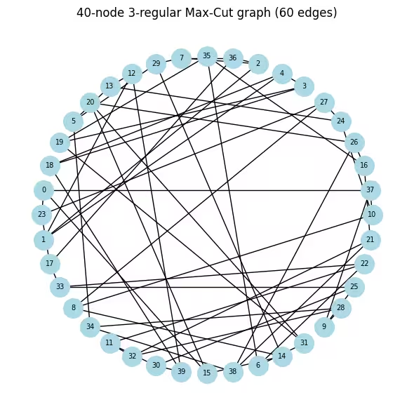
Cost operator: 40 qubits, 60 Pauli terms
c* range: [0.000, 1.000]  theta range: [1.047, 2.094] rad

Transpiled circuit: 2Q depth=86

# ── Classical baseline via simulated annealing ────────────────────
# Run SA before any hardware calls to get a strong classical reference cut
# value. SA is fast (seconds), needs no solver license, and reliably finds
# near-optimal solutions on 40-node graphs. We use sa_cut as the denominator
# for the approximation ratio instead of the looser QP upper bound.
#
# At each step we flip a random node and accept the move if it improves the
# cut, or with probability exp(delta/T) otherwise. Temperature T decays
# geometrically, allowing uphill moves early on to escape local minima.
def simulated_annealing_maxcut(
    G, seed=0, T0=2.0, T_min=1e-4, alpha=0.995, n_steps=100_000
):
    rng_sa = np.random.default_rng(seed)
    n = G.number_of_nodes()
    x = rng_sa.integers(0, 2, n)
    best_x = x.copy()
    best_cut = sum(1 for u, v in G.edges() if x[u] != x[v])
    T = T0
    for _ in range(n_steps):
        i = rng_sa.integers(0, n)
        delta = sum((-1 if x[i] != x[nb] else 1) for nb in G.neighbors(i))
        if delta > 0 or rng_sa.random() < np.exp(delta / T):
            x[i] ^= 1
            cut = sum(1 for u, v in G.edges() if x[u] != x[v])
            if cut > best_cut:
                best_cut, best_x = cut, x.copy()
        T = max(T * alpha, T_min)
    return best_x, best_cut

sa_solution, sa_cut = simulated_annealing_maxcut(G_large)
print(f"Simulated annealing cut value: {sa_cut}  (classical reference)")

# ── Step 3: Execution on hardware ───────────────────────────
# A Session reserves the backend so the COBYLA iterations and final sampling
# run back-to-back without re-queuing between jobs — important when the
# optimizer submits many short jobs sequentially. All jobs are tagged with
# "TUT_WSQAOA" for traceability in the IBM Quantum dashboard.
#
# EstimatorV2 with resilience_level=1 enables twirled readout error extinction
# (TREX), which corrects systematic measurement bit-flip errors without extra
# circuit overhead. 4096 shots per call balances estimation noise vs. job time.
estimator_options = EstimatorOptions()
estimator_options.resilience_level = 1
estimator_options.default_shots = 4096
estimator_options.environment.job_tags = ["TUT_WSQAOA"]

# Align the cost observable with the physical qubit layout chosen by the transpiler
cost_op_isa = cost_op_large.apply_layout(ws_isa_large.layout)
ws_param_order_isa = list(ws_isa_large.parameters)

ws_history_hw = []

with Session(backend=backend) as session:
    estimator_hw = Estimator(mode=session, options=estimator_options)

    def hw_cost_fn(params):
        bound = ws_isa_large.assign_parameters(
            dict(zip(ws_param_order_isa, params))
        )
        energy = (
            estimator_hw.run([(bound, cost_op_isa)]).result()[0].data.evs.real
        )
        ws_history_hw.append(float(energy))
        print(
            f"  iter {len(ws_history_hw):>3d}  <H_C> = {energy:.4f}", end="\r"
        )
        return float(energy)

    # Warm-start initialization: gamma=0 means the cost unitary is the identity on
    # the first call, so COBYLA immediately evaluates the warm-start state itself —
    # a much better starting signal than a random point.
    ws_params0_hw = np.concatenate(
        [np.zeros(p_large), np.full(p_large, np.pi / 4)]
    )

    ws_result_hw = minimize(
        hw_cost_fn,
        ws_params0_hw,
        method="COBYLA",
        options={"maxiter": 150, "rhobeg": 0.3},
    )
    print(
        f"\nOptimization complete: energy={ws_result_hw.fun:.4f}, "
        f"iterations={len(ws_history_hw)}"
    )

    # ── Step 3b: Sample the optimized circuit ──────────────────────────────────
    # Use 8192 shots for the final sample to get a reliable mode estimate.
    sampler_hw = Sampler(
        mode=session,
        options={"environment": {"job_tags": ["TUT_WSQAOA"]}},
    )
    ws_bound_hw = ws_isa_large.assign_parameters(
        dict(zip(ws_param_order_isa, ws_result_hw.x))
    )
    counts_hw = (
        sampler_hw.run([ws_bound_hw], shots=8192)
        .result()[0]
        .data.meas.get_counts()
    )

best_bs_hw = max(counts_hw, key=counts_hw.get)
best_count = counts_hw[best_bs_hw]
total_shots = sum(counts_hw.values())

# Decode: Qiskit returns bitstrings with qubit 0 at the rightmost position,
# so reversing the string maps character index i to variable x_i.
cut_val_hw, s0_hw, s1_hw = evaluate_cut(best_bs_hw[::-1], G_large)

# Compare against simulated annealing.
# A ratio >= 1.0 means WS-QAOA matched or beat the classical SA solution.
# A ratio close to 1.0 (e.g. > 0.95) shows the quantum result is competitive.
approx_ratio_hw = cut_val_hw / sa_cut
print(
    f"Most-probable bitstring frequency: {best_count}/{total_shots} "
    f"({100*best_count/total_shots:.1f}%)"
)
print(
    f"WS-QAOA cut: {cut_val_hw}  |  SA cut: {sa_cut}  "
    f"|  Approximation ratio vs SA: {approx_ratio_hw:.4f}"
)

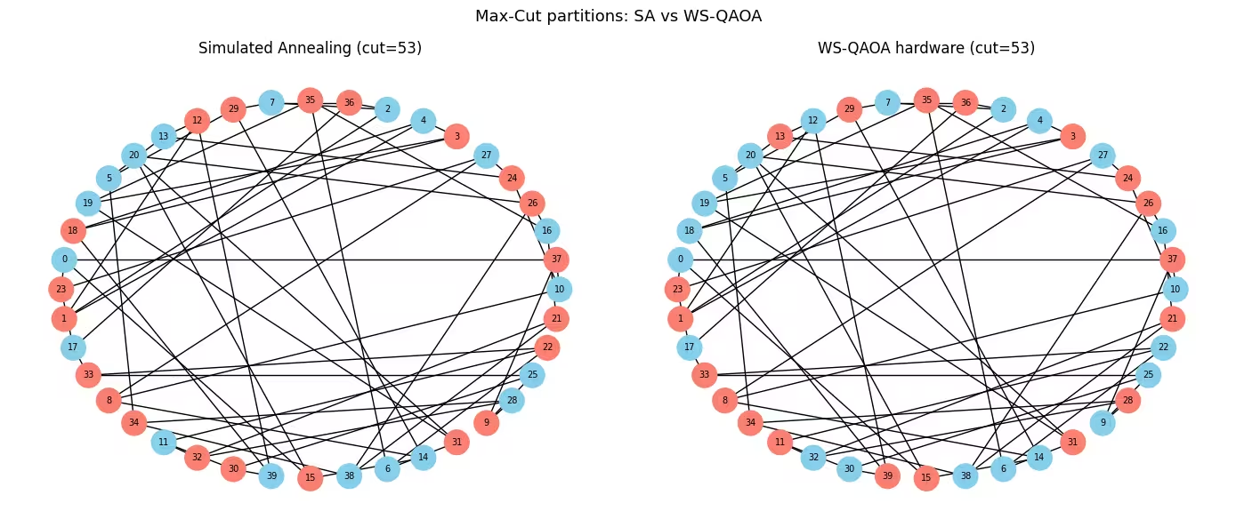
# Visualize both solutions side-by-side on the graph.
# Blue = partition S, orange = partition S-bar.
# Edges crossing between colors are the ones counted in the cut.
fig, axes = plt.subplots(1, 2, figsize=(14, 6))
for ax, assignment, cut, title in [
    (
        axes[0],
        list(sa_solution),
        sa_cut,
        f"Simulated Annealing (cut={sa_cut})",
    ),
    (
        axes[1],
        [int(b) for b in best_bs_hw[::-1]],
        cut_val_hw,
        f"WS-QAOA hardware (cut={cut_val_hw})",
    ),
]:
    colors = [
        "skyblue" if assignment[i] == 0 else "salmon" for i in G_large.nodes()
    ]
    nx.draw(
        G_large,
        pos_large,
        with_labels=True,
        node_color=colors,
        node_size=400,
        font_size=7,
        ax=ax,
    )
    ax.set_title(title)
plt.suptitle("Max-Cut partitions: SA vs WS-QAOA", fontsize=13)
plt.tight_layout()
plt.show()

# ── Step 4: Convergence plot and summary ──────────────────────────────────
# On real hardware the trace will be noisy (shot noise + gate errors), but the
# overall downward trend confirms that COBYLA is making progress despite noise.
fig, ax = plt.subplots(figsize=(7, 4))
ax.plot(ws_history_hw, color="tab:orange", label="WS-QAOA (hardware)")
ax.axhline(
    ws_result_hw.fun,
    color="tab:orange",
    linestyle=":",
    label=f"Final energy ({ws_result_hw.fun:.3f})",
)
ax.set_xlabel("Optimizer call")
ax.set_ylabel(r"$\langle H_C \rangle$")
ax.set_title(f"WS-QAOA convergence on {backend.name} (40 qubits, p=1)")
ax.legend()
plt.tight_layout()
plt.show()

print("\n=== Large Scale Summary ===")
print(f"{'Metric':<38} {'Value':>10}")
print("-" * 50)
print(f"{'Nodes / Edges':<38} {N_LARGE:>5} / {len(edges_large):<4}")
print(f"{'QAOA layers (p)':<38} {p_large:>10}")
print(f"{'Transpiled ECR gate count':<38} {ecr_count:>10}")
print(f"{'Transpiled circuit depth':<38} {ws_isa_large.depth():>10}")
print(f"{'Optimizer iterations':<38} {len(ws_history_hw):>10}")
print(f"{'WS-QAOA energy (hardware)':<38} {ws_result_hw.fun:>10.4f}")
print(f"{'Cut value':<38} {cut_val_hw:>10}")
print(f"{'Simulated annealing cut value':<38} {sa_cut:>10}")
print(f"{'Approximation ratio (vs SA)':<38} {approx_ratio_hw:>10.4f}")

Simulated annealing cut value: 53  (classical reference)
  iter  31  <H_C> = -12.4094
Optimization complete: energy=-13.0256, iterations=31
Most-probable bitstring frequency: 4/8192 (0.0%)
WS-QAOA cut: 53  |  SA cut: 53  |  Approximation ratio vs SA: 1.0000

=== Large Scale Summary ===
Metric                                      Value
--------------------------------------------------
Nodes / Edges                             40 / 60  
QAOA layers (p)                                 1
Transpiled ECR gate count                       0
Transpiled circuit depth                      276
Optimizer iterations                           31
WS-QAOA energy (hardware)                -13.0256
Cut value                                      53
Simulated annealing cut value                  53
Approximation ratio (vs SA)                1.0000

Próximos pasos

Recomendaciones

Si este trabajo te resultó interesante, podrían interesarte los siguientes materiales:

• Capas superiores de QAOA: Aumenta p para ver cómo ambos algoritmos mejoran con más capas de circuito, y si la ventaja de WS-QAOA a baja profundidad persiste.
• Mapeador de optimización del complemento Qiskit: Explora la documentación e intenta modelar diferentes problemas combinatorios, o usar diferentes solucionadores para la relajación continua.

Referencias

[1] D. J. Egger, J. Mareček, and S. Woerner, "Warm-starting quantum optimization," Quantum, vol. 5, p. 479, 2021. arXiv:2009.10095

[2] E. Farhi, J. Goldstone, and S. Gutmann, "A quantum approximate optimization algorithm," arXiv:1411.4028, 2014.