Métodos de compilación para circuitos de simulación hamiltoniana
Estimación de uso: menos de 1 minuto en un procesador IBM Heron (NOTA: Solo es una estimación. Tu tiempo de ejecución puede variar.)
Resultados de aprendizaje
Después de completar este tutorial, comprenderás:
- Cómo usar el transpilador de Qiskit con SABRE para la optimización de distribución y enrutamiento
- Cómo aprovechar el transpilador potenciado por IA para la optimización avanzada de circuitos
- Cómo usar el plugin Rustiq para sintetizar operaciones
PauliEvolutionGateen circuitos de simulación hamiltoniana - Cómo comparar métodos de compilación usando la profundidad de dos qubits, el número total de compuertas y el tiempo de ejecución
Requisitos previos
Te sugerimos que estés familiarizado con los siguientes temas antes de comenzar este tutorial:
Contexto
La compilación de circuitos cuánticos transforma un algoritmo cuántico de alto nivel en un circuito físico que respeta las restricciones del hardware objetivo. Una compilación eficaz puede reducir significativamente la profundidad del circuito y el número de compuertas, ambos de los cuales impactan directamente en la calidad de los resultados en dispositivos cuánticos de corto plazo.
Este tutorial compara tres métodos de compilación en circuitos de simulación hamiltoniana construidos con PauliEvolutionGate. Estos circuitos modelan interacciones por pares entre qubits (como términos , e ) y son comunes en química cuántica, física de materia condensada y ciencia de materiales.
Los circuitos de la comparación provienen de la colección Hamlib, a la que se accede a través del repositorio Benchpress. Hamlib proporciona un conjunto estandarizado de hamiltonianos representativos, lo que permite comparar estrategias de compilación en cargas de trabajo de simulación realistas.
Descripción general de los métodos de compilación
Transpilador de Qiskit con SABRE
El transpilador de Qiskit usa el algoritmo SABRE (SWAP-based BidiREctional heuristic search) para optimizar la distribución y el enrutamiento del circuito. SABRE se enfoca en minimizar las compuertas SWAP y su impacto en la profundidad del circuito, respetando las restricciones de conectividad del hardware. Es un método de propósito general que ofrece un buen equilibrio entre rendimiento y tiempo de compilación. Para más detalles, consulta [1]. Las ventajas y la exploración de parámetros de SABRE se cubren en profundidad en un tutorial separado.
Transpilador potenciado por IA
El transpilador potenciado por IA usa aprendizaje automático para predecir estrategias óptimas de transpilación, analizando patrones en la estructura del circuito y las restricciones del hardware. También puede aplicar el pase AIPauliNetworkSynthesis, que se dirige a circuitos de redes de Pauli usando un enfoque de síntesis basado en aprendizaje por refuerzo. Para más información, consulta [2] y [3].
Plugin Rustiq
El plugin Rustiq proporciona técnicas avanzadas de síntesis específicamente para operaciones PauliEvolutionGate, que representan rotaciones de Pauli comúnmente utilizadas en dinámicas trotterizadas. Está diseñado para producir descomposiciones de circuito de baja profundidad para cargas de trabajo de simulación hamiltoniana. Para más detalles, consulta [4].
Métricas clave
Comparamos los tres métodos en las siguientes métricas:
- Profundidad de dos qubits: La profundidad del circuito contando solo las compuertas de dos qubits. Este suele ser el cuello de botella para la fidelidad en hardware real.
- Tamaño del circuito (número total de compuertas): El número total de compuertas en el circuito transpilado.
- Tiempo de ejecución: El tiempo de reloj para la transpilación.
Requisitos
Antes de comenzar este tutorial, asegúrate de tener instalado lo siguiente:
- Qiskit SDK v2.0 o posterior, con soporte de visualización
- Qiskit Runtime v0.22 o posterior (
pip install qiskit-ibm-runtime) - Qiskit Aer (
pip install qiskit-aer) - Qiskit IBM Transpiler (
pip install qiskit-ibm-transpiler) - Modo local del transpilador de IA de Qiskit (
pip install qiskit_ibm_ai_local_transpiler) - Networkx (
pip install networkx)
Configuración
# Added by doQumentation — required packages for this notebook
!pip install -q matplotlib numpy qiskit qiskit-aer qiskit-ibm-runtime qiskit-ibm-transpiler requests scipy
from qiskit.circuit import QuantumCircuit
from qiskit_ibm_runtime import QiskitRuntimeService, SamplerV2
from qiskit.circuit.library import PauliEvolutionGate
from qiskit_ibm_transpiler import generate_ai_pass_manager
from qiskit.quantum_info import SparsePauliOp
from qiskit.transpiler.preset_passmanagers import generate_preset_pass_manager
from qiskit.transpiler.passes.synthesis.high_level_synthesis import HLSConfig
from qiskit_aer import AerSimulator
from qiskit_aer.noise import NoiseModel, depolarizing_error
from collections import Counter
from statistics import mean, stdev
from scipy.sparse import SparseEfficiencyWarning
import time
import warnings
import matplotlib.pyplot as plt
import matplotlib.ticker as ticker
import numpy as np
import json
import requests
import logging

# Suppress noisy loggers and warnings
logging.getLogger(
    "qiskit_ibm_transpiler.wrappers.ai_local_synthesis"
).setLevel(logging.ERROR)
warnings.filterwarnings("ignore", category=FutureWarning)
warnings.filterwarnings("ignore", category=SparseEfficiencyWarning)

seed = 42  # Seed for reproducibility
Conectarse a un backend
Selecciona un backend que se utilizará tanto para los ejemplos de pequeña como de gran escala. El backend determina el mapa de acoplamiento y las compuertas base a las que apunta el transpilador.
# QiskitRuntimeService.save_account(channel="ibm_quantum_platform",
# token="<YOUR-API-KEY>", overwrite=True, set_as_default=True)
service = QiskitRuntimeService(channel="ibm_quantum_platform")
backend = service.least_busy(operational=True, simulator=False)
print(f"Using backend: {backend.name}")
Using backend: ibm_pittsburgh
Definir gestores de pases
Configura los tres métodos de compilación.
# SABRE pass manager (Qiskit default at optimization level 3)
pm_sabre = generate_preset_pass_manager(
    optimization_level=3, backend=backend, seed_transpiler=seed
)
# AI transpiler pass manager (local mode)
pm_ai = generate_ai_pass_manager(
    backend=backend, optimization_level=3, ai_optimization_level=3
)
Fetching 127 files: 0%| | 0/127 [00:00<?, ?it/s]
# Rustiq pass manager for PauliEvolutionGate synthesis
hls_config = HLSConfig(
    PauliEvolution=[
        (
            "rustiq",
            {
                "nshuffles": 400,
                "upto_phase": True,
                "fix_clifford": True,
                "preserve_order": False,
                "metric": "depth",
            },
        )
    ]
)
pm_rustiq = generate_preset_pass_manager(
    optimization_level=3,
    backend=backend,
    hls_config=hls_config,
    seed_transpiler=seed,
)
Definir funciones auxiliares
La siguiente función transpila una lista de circuitos usando un gestor de pases dado y registra las métricas clave (profundidad de dos qubits, tamaño del circuito y tiempo de ejecución) para cada circuito.
def capture_transpilation_metrics(
    results, pass_manager, circuits, method_name
):
    """
    Transpile circuits and append one metrics record per circuit to
    ``results``.

    Args:
        results (list): List of dicts to append the metrics records to.
        pass_manager: Pass manager used for transpilation.
        circuits (list): List of quantum circuits to transpile.
        method_name (str): Name of the transpilation method.

    Returns:
        list: List of transpiled circuits.
    """
    transpiled_circuits = []

    for i, qc in enumerate(circuits):
        start_time = time.time()
        transpiled_qc = pass_manager.run(qc)
        end_time = time.time()

        # Decompose swaps for consistency across methods
        transpiled_qc = transpiled_qc.decompose(gates_to_decompose=["swap"])

        transpilation_time = end_time - start_time
        two_qubit_depth = transpiled_qc.depth(
            lambda x: x.operation.num_qubits == 2
        )
        circuit_size = transpiled_qc.size()

        results.append(
            {
                "method": method_name,
                "qc_name": qc.name,
                "qc_index": i,
                "num_qubits": qc.num_qubits,
                "two_qubit_depth": two_qubit_depth,
                "size": circuit_size,
                "runtime": transpilation_time,
            }
        )
        transpiled_circuits.append(transpiled_qc)
        print(
            f"[{method_name}] Circuit {i} ({qc.name}): "
            f"2Q depth={two_qubit_depth}, size={circuit_size}, "
            f"time={transpilation_time:.2f}s"
        )

    return transpiled_circuits
def _method_order(results):
    """Return the distinct method names in their first-seen order."""
    order = []
    for r in results:
        if r["method"] not in order:
            order.append(r["method"])
    return order

def print_summary_table(results):
    """
    Print the mean and standard deviation of each metric per compilation
    method, followed by the mean percent improvement relative to SABRE.
    """
    metrics = [
        ("two_qubit_depth", "2Q Depth"),
        ("size", "Gate Count"),
        ("runtime", "Runtime (s)"),
    ]
    methods = _method_order(results)
    by_method = {m: [r for r in results if r["method"] == m] for m in methods}
    sabre_by_index = {r["qc_index"]: r for r in by_method.get("SABRE", [])}

    col_w = 22
    name_w = max(len(m) for m in methods)
    header = f"{'Method':<{name_w}}" + "".join(
        f"  {label:>{col_w}}" for _, label in metrics
    )

    print("Mean +/- std per compilation method")
    print(header)
    print("-" * len(header))
    for method in methods:
        cells = []
        for key, _ in metrics:
            values = [r[key] for r in by_method[method]]
            std = stdev(values) if len(values) > 1 else 0.0
            cells.append(f"{mean(values):,.1f} +/- {std:,.1f}")
        print(
            f"{method:<{name_w}}" + "".join(f"  {c:>{col_w}}" for c in cells)
        )

    others = [m for m in methods if m != "SABRE"]
    if others and sabre_by_index:
        print()
        print("Mean % improvement vs SABRE (positive = better than SABRE)")
        print(header)
        print("-" * len(header))
        for method in others:
            cells = []
            for key, _ in metrics:
                pct = [
                    (sabre_by_index[r["qc_index"]][key] - r[key])
                    / sabre_by_index[r["qc_index"]][key]
                    * 100
                    for r in by_method[method]
                    if sabre_by_index.get(r["qc_index"])
                    and sabre_by_index[r["qc_index"]][key]
                ]
                if pct:
                    std = stdev(pct) if len(pct) > 1 else 0.0
                    cells.append(f"{mean(pct):+.1f}% +/- {std:.1f}%")
                else:
                    cells.append("n/a")
            print(
                f"{method:<{name_w}}"
                + "".join(f"  {c:>{col_w}}" for c in cells)
            )
def print_per_circuit_comparison(results, num_rows=5):
    """
    Print a per-metric comparison of the compilation methods for the
    first ``num_rows`` circuits (sorted by qubit count). The best
    (lowest) value for each metric is marked with an asterisk.
    """
    metrics = [
        ("two_qubit_depth", "2Q Depth"),
        ("size", "Gate Count"),
        ("runtime", "Runtime (s)"),
    ]
    methods = _method_order(results)

    by_index = {}
    for r in results:
        by_index.setdefault(r["qc_index"], {})[r["method"]] = r
    ordered = sorted(
        by_index.items(),
        key=lambda kv: (next(iter(kv[1].values()))["num_qubits"], kv[0]),
    )[:num_rows]

    for key, label in metrics:
        print(f"{label} (first {num_rows} circuits by qubit count); * = best")
        header = f"{'Idx':>3}  {'Circuit':<16} {'Q':>3}" + "".join(
            f"{m:>9}" for m in methods
        )
        print(header)
        print("-" * len(header))
        for idx, method_map in ordered:
            any_record = next(iter(method_map.values()))
            present = {
                m: method_map[m][key] for m in methods if m in method_map
            }
            best = min(present.values())
            line = (
                f"{idx:>3}  {any_record['qc_name'][:16]:<16} "
                f"{any_record['num_qubits']:>3}"
            )
            for m in methods:
                value = method_map[m][key]
                text = f"{value:.2f}" if key == "runtime" else f"{int(value)}"
                if value == best:
                    text += "*"
                line += f"{text:>9}"
            print(line)
        print()
Cargar circuitos hamiltonianos desde Hamlib
Cargamos un conjunto representativo de hamiltonianos del repositorio Benchpress y construimos circuitos con PauliEvolutionGate. Se eliminan los circuitos que superan el número de qubits del backend, así como aquellos cuyo tamaño descompuesto excede las 1.500 compuertas (para mantener los tiempos de transpilación razonables).
# Obtain the Hamiltonian JSON from the benchpress repository
url = "https://raw.githubusercontent.com/Qiskit/benchpress/e7b29ef7be4cc0d70237b8fdc03edbd698908eff/benchpress/hamiltonian/hamlib/100_representative.json"
response = requests.get(url)
response.raise_for_status()
ham_records = json.loads(response.text)

# Remove circuits that are too large for the backend
ham_records = [
    h for h in ham_records if h["ham_qubits"] <= backend.num_qubits
]

# Build PauliEvolutionGate circuits
qc_ham_list = []
for h in ham_records:
    terms = h["ham_hamlib_hamiltonian_terms"]
    coeff = h["ham_hamlib_hamiltonian_coefficients"]
    num_qubits = h["ham_qubits"]
    name = h["ham_problem"]

    evo_gate = PauliEvolutionGate(SparsePauliOp(terms, coeff))
    qc = QuantumCircuit(num_qubits)
    qc.name = name
    qc.append(evo_gate, range(num_qubits))
    qc_ham_list.append(qc)

# Remove circuits whose decomposed size exceeds 1500 gates so that transpilation completes in a reasonable time frame
qc_ham_list = [qc for qc in qc_ham_list if qc.decompose().size() <= 1500]

print(f"Total Hamiltonian circuits loaded: {len(qc_ham_list)}")
print(
    f"Qubit range: {min(qc.num_qubits for qc in qc_ham_list)} to {max(qc.num_qubits for qc in qc_ham_list)}"
)
Total Hamiltonian circuits loaded: 42
Qubit range: 2 to 112
Divide los circuitos en grupos de pequeña escala (menos de 20 qubits) y gran escala (20 o más qubits).
qc_small = [qc for qc in qc_ham_list if qc.num_qubits < 20]
qc_large = [qc for qc in qc_ham_list if qc.num_qubits >= 20]

print(f"Small-scale circuits (<20 qubits): {len(qc_small)}")
print(f"Large-scale circuits (>=20 qubits): {len(qc_large)}")
Small-scale circuits (<20 qubits): 20
Large-scale circuits (>=20 qubits): 22
Previsualiza uno de los circuitos hamiltonianos de pequeña escala antes de la transpilación.
# We decompose the circuit here, otherwise it would just be a PauliEvolutionGate box,
# which isn't very informative to look at!
qc_small[0].decompose().draw("mpl", fold=-1)

Ejemplo de pequeña escala
En esta sección, comparamos los tres métodos de compilación en circuitos hamiltonianos con menos de 20 qubits. Estos circuitos se transpilar rápidamente y ofrecen una visión clara de cómo cada método maneja circuitos de complejidad moderada.
Paso 1: Mapear entradas clásicas a un problema cuántico
Cada hamiltoniano se codifica como un circuito con PauliEvolutionGate. Los circuitos ya se construyeron en la sección de configuración a partir de los datos de la comparación de Hamlib.
Paso 2: Optimizar el problema para la ejecución en hardware cuántico
Transpilamos todos los circuitos de pequeña escala usando cada uno de los tres gestores de pases y recopilamos las métricas.
results_small = []

tqc_sabre_small = capture_transpilation_metrics(
    results_small, pm_sabre, qc_small, "SABRE"
)
tqc_ai_small = capture_transpilation_metrics(
    results_small, pm_ai, qc_small, "AI"
)
tqc_rustiq_small = capture_transpilation_metrics(
    results_small, pm_rustiq, qc_small, "Rustiq"
)
[SABRE] Circuit 0 (all-vib-bh): 2Q depth=3, size=30, time=2.09s
[SABRE] Circuit 1 (all-vib-c2h): 2Q depth=18, size=111, time=0.01s
[SABRE] Circuit 2 (all-vib-o3): 2Q depth=6, size=58, time=0.00s
[SABRE] Circuit 3 (all-vib-c2h): 2Q depth=2, size=37, time=0.01s
[SABRE] Circuit 4 (graph-gnp_k-2): 2Q depth=24, size=126, time=0.01s
[SABRE] Circuit 5 (LiH): 2Q depth=66, size=285, time=0.01s
[SABRE] Circuit 6 (all-vib-fccf): 2Q depth=66, size=339, time=0.01s
[SABRE] Circuit 7 (all-vib-ch2): 2Q depth=88, size=413, time=0.01s
[SABRE] Circuit 8 (all-vib-f2): 2Q depth=180, size=1000, time=0.02s
[SABRE] Circuit 9 (all-vib-bhf2): 2Q depth=18, size=223, time=0.03s
[SABRE] Circuit 10 (graph-gnp_k-4): 2Q depth=122, size=675, time=0.02s
[SABRE] Circuit 11 (Be2): 2Q depth=343, size=1628, time=0.03s
[SABRE] Circuit 12 (all-vib-fccf): 2Q depth=14, size=134, time=0.00s
[SABRE] Circuit 13 (uf20-ham): 2Q depth=50, size=341, time=0.01s
[SABRE] Circuit 14 (TSP_Ncity-4): 2Q depth=118, size=615, time=0.01s
[SABRE] Circuit 15 (graph-complete_bipart): 2Q depth=232, size=1420, time=0.03s
[SABRE] Circuit 16 (all-vib-cyclo_propene): 2Q depth=18, size=354, time=0.93s
[SABRE] Circuit 17 (all-vib-hno): 2Q depth=6, size=174, time=0.14s
[SABRE] Circuit 18 (all-vib-fccf): 2Q depth=30, size=286, time=0.01s
[SABRE] Circuit 19 (tfim): 2Q depth=31, size=232, time=0.03s
[AI] Circuit 0 (all-vib-bh): 2Q depth=3, size=30, time=0.01s
Fetching 4 files: 0%| | 0/4 [00:00<?, ?it/s]
[AI] Circuit 1 (all-vib-c2h): 2Q depth=18, size=101, time=0.18s
[AI] Circuit 2 (all-vib-o3): 2Q depth=6, size=58, time=0.01s
[AI] Circuit 3 (all-vib-c2h): 2Q depth=2, size=37, time=0.01s
[AI] Circuit 4 (graph-gnp_k-2): 2Q depth=24, size=133, time=0.07s
[AI] Circuit 5 (LiH): 2Q depth=62, size=267, time=8.00s
[AI] Circuit 6 (all-vib-fccf): 2Q depth=65, size=300, time=0.18s
[AI] Circuit 7 (all-vib-ch2): 2Q depth=79, size=353, time=0.16s
[AI] Circuit 8 (all-vib-f2): 2Q depth=176, size=998, time=0.43s
[AI] Circuit 9 (all-vib-bhf2): 2Q depth=18, size=194, time=0.11s
[AI] Circuit 10 (graph-gnp_k-4): 2Q depth=114, size=668, time=0.18s
[AI] Circuit 11 (Be2): 2Q depth=292, size=1382, time=0.88s
[AI] Circuit 12 (all-vib-fccf): 2Q depth=14, size=134, time=0.01s
[AI] Circuit 13 (uf20-ham): 2Q depth=40, size=330, time=0.16s
[AI] Circuit 14 (TSP_Ncity-4): 2Q depth=96, size=600, time=0.29s
[AI] Circuit 15 (graph-complete_bipart): 2Q depth=231, size=1531, time=0.46s
[AI] Circuit 16 (all-vib-cyclo_propene): 2Q depth=18, size=309, time=0.25s
[AI] Circuit 17 (all-vib-hno): 2Q depth=10, size=198, time=0.15s
[AI] Circuit 18 (all-vib-fccf): 2Q depth=34, size=402, time=0.02s
[AI] Circuit 19 (tfim): 2Q depth=44, size=311, time=0.15s
[Rustiq] Circuit 0 (all-vib-bh): 2Q depth=3, size=30, time=0.01s
[Rustiq] Circuit 1 (all-vib-c2h): 2Q depth=13, size=69, time=0.00s
[Rustiq] Circuit 2 (all-vib-o3): 2Q depth=13, size=82, time=0.01s
[Rustiq] Circuit 3 (all-vib-c2h): 2Q depth=2, size=40, time=0.01s
[Rustiq] Circuit 4 (graph-gnp_k-2): 2Q depth=31, size=132, time=0.01s
[Rustiq] Circuit 5 (LiH): 2Q depth=59, size=285, time=0.01s
[Rustiq] Circuit 6 (all-vib-fccf): 2Q depth=34, size=193, time=0.00s
[Rustiq] Circuit 7 (all-vib-ch2): 2Q depth=49, size=302, time=0.01s
[Rustiq] Circuit 8 (all-vib-f2): 2Q depth=141, size=807, time=0.02s
[Rustiq] Circuit 9 (all-vib-bhf2): 2Q depth=13, size=146, time=0.02s
[Rustiq] Circuit 10 (graph-gnp_k-4): 2Q depth=129, size=683, time=0.02s
[Rustiq] Circuit 11 (Be2): 2Q depth=220, size=1101, time=0.02s
[Rustiq] Circuit 12 (all-vib-fccf): 2Q depth=53, size=333, time=0.01s
[Rustiq] Circuit 13 (uf20-ham): 2Q depth=63, size=425, time=0.01s
[Rustiq] Circuit 14 (TSP_Ncity-4): 2Q depth=123, size=767, time=0.02s
[Rustiq] Circuit 15 (graph-complete_bipart): 2Q depth=309, size=2107, time=0.05s
[Rustiq] Circuit 16 (all-vib-cyclo_propene): 2Q depth=16, size=283, time=0.32s
[Rustiq] Circuit 17 (all-vib-hno): 2Q depth=19, size=291, time=0.32s
[Rustiq] Circuit 18 (all-vib-fccf): 2Q depth=44, size=546, time=0.02s
[Rustiq] Circuit 19 (tfim): 2Q depth=24, size=416, time=0.01s
La siguiente tabla resume el promedio y la desviación estándar de cada métrica en todos los circuitos de pequeña escala, junto con el porcentaje de mejora relativo a SABRE. Dado que los tamaños de los circuitos varían ampliamente, la desviación estándar proporciona contexto importante para interpretar los promedios.
print_summary_table(results_small)
Mean +/- std per compilation method
Method                2Q Depth              Gate Count             Runtime (s)
------------------------------------------------------------------------------
SABRE            71.8 +/- 89.6         424.1 +/- 446.0             0.2 +/- 0.5
AI               67.3 +/- 80.2         416.8 +/- 426.7             0.6 +/- 1.8
Rustiq           67.9 +/- 80.0         451.9 +/- 484.7             0.0 +/- 0.1

Mean % improvement vs SABRE (positive = better than SABRE)
Method                2Q Depth              Gate Count             Runtime (s)
------------------------------------------------------------------------------
AI             -2.1% +/- 19.8%         -0.6% +/- 14.7%   -5635.1% +/- 20725.2%
Rustiq        -25.3% +/- 85.4%        -16.3% +/- 50.4%         -7.0% +/- 60.6%
La tabla por circuito muestra cómo se compara cada método en circuitos individuales. El mejor valor para cada métrica está marcado con un asterisco. Observa que para los circuitos más simples, los tres métodos a menudo convergen al mismo resultado.
print_per_circuit_comparison(results_small, num_rows=8)
2Q Depth (first 8 circuits by qubit count); * = best
Idx  Circuit            Q    SABRE       AI   Rustiq
----------------------------------------------------
  0  all-vib-bh         2       3*       3*       3*
  1  all-vib-c2h        3       18       18      13*
  2  all-vib-o3         4       6*       6*       13
  3  all-vib-c2h        4       2*       2*       2*
  4  graph-gnp_k-2      4      24*      24*       31
  5  LiH                4       66       62      59*
  6  all-vib-fccf       4       66       65      34*
  7  all-vib-ch2        4       88       79      49*

Gate Count (first 8 circuits by qubit count); * = best
Idx  Circuit            Q    SABRE       AI   Rustiq
----------------------------------------------------
  0  all-vib-bh         2      30*      30*      30*
  1  all-vib-c2h        3      111      101      69*
  2  all-vib-o3         4      58*      58*       82
  3  all-vib-c2h        4      37*      37*       40
  4  graph-gnp_k-2      4     126*      133      132
  5  LiH                4      285     267*      285
  6  all-vib-fccf       4      339      300     193*
  7  all-vib-ch2        4      413      353     302*

Runtime (s) (first 8 circuits by qubit count); * = best
Idx  Circuit            Q    SABRE       AI   Rustiq
----------------------------------------------------
  0  all-vib-bh         2     2.09     0.01    0.01*
  1  all-vib-c2h        3     0.01     0.18    0.00*
  2  all-vib-o3         4    0.00*     0.01     0.01
  3  all-vib-c2h        4     0.01     0.01    0.01*
  4  graph-gnp_k-2      4    0.01*     0.07     0.01
  5  LiH                4    0.01*     8.00     0.01
  6  all-vib-fccf       4     0.01     0.18    0.00*
  7  all-vib-ch2        4     0.01     0.16    0.01*
Visualizar resultados
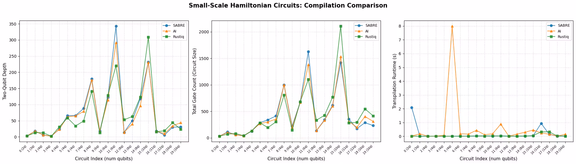
Los gráficos a continuación comparan los tres métodos en cada métrica por circuito. Los circuitos están ordenados por número de qubits y etiquetados por índice en el eje x, ya que múltiples circuitos pueden compartir el mismo número de qubits.
def plot_transpilation_comparison(results, title_prefix):
    """
    Create a three-panel figure comparing compilation methods on
    two-qubit depth, circuit size, and runtime.

    Circuits are sorted by qubit count and plotted by circuit index.
    """
    methods = _method_order(results)
    palette = {"SABRE": "#1f77b4", "AI": "#ff7f0e", "Rustiq": "#2ca02c"}
    markers = {"SABRE": "o", "AI": "^", "Rustiq": "s"}

    # Order circuits by qubit count (then index) and map to plot positions
    ref = sorted(
        [r for r in results if r["method"] == methods[0]],
        key=lambda r: (r["num_qubits"], r["qc_index"]),
    )
    pos_map = {r["qc_index"]: pos for pos, r in enumerate(ref)}
    tick_positions = [pos_map[r["qc_index"]] for r in ref]
    tick_labels = [
        f"{pos_map[r['qc_index']]} ({r['num_qubits']}q)" for r in ref
    ]

    metrics = [
        ("two_qubit_depth", "Two-Qubit Depth"),
        ("size", "Total Gate Count (Circuit Size)"),
        ("runtime", "Transpilation Runtime (s)"),
    ]

    fig, axes = plt.subplots(1, 3, figsize=(20, 5.5))
    fig.suptitle(title_prefix, fontsize=15, fontweight="bold", y=1.02)

    for ax, (metric, ylabel) in zip(axes, metrics):
        for method in methods:
            subset = sorted(
                [r for r in results if r["method"] == method],
                key=lambda r: pos_map[r["qc_index"]],
            )
            ax.plot(
                [pos_map[r["qc_index"]] for r in subset],
                [r[metric] for r in subset],
                marker=markers.get(method, "o"),
                label=method,
                color=palette.get(method, None),
                linewidth=1.5,
                markersize=6,
                alpha=0.85,
            )
        ax.set_xlabel("Circuit Index (num qubits)", fontsize=11)
        ax.set_ylabel(ylabel, fontsize=11)
        ax.legend(frameon=True, fontsize=9)
        ax.grid(True, linestyle="--", alpha=0.4)
        step = max(1, len(tick_positions) // 15)
        ax.set_xticks(tick_positions[::step])
        ax.set_xticklabels(
            [tick_labels[i] for i in range(0, len(tick_labels), step)],
            fontsize=7,
            rotation=45,
            ha="right",
        )

    plt.tight_layout()
    plt.show()
def plot_pct_improvement_vs_sabre(results, title_prefix):
    """
    Plot the per-circuit percent improvement of each non-SABRE method
    relative to SABRE, for each metric. A positive value means the
    method improved on SABRE; negative means SABRE was better.
    """
    metrics = [
        ("two_qubit_depth", "2Q Depth"),
        ("size", "Gate Count"),
        ("runtime", "Runtime"),
    ]
    palette = {"AI": "#ff7f0e", "Rustiq": "#2ca02c"}
    markers = {"AI": "^", "Rustiq": "s"}

    methods = _method_order(results)
    sabre = sorted(
        [r for r in results if r["method"] == "SABRE"],
        key=lambda r: (r["num_qubits"], r["qc_index"]),
    )
    other_methods = [m for m in methods if m != "SABRE"]

    tick_positions = list(range(len(sabre)))
    tick_labels = [
        f"{i} ({sabre[i]['num_qubits']}q)" for i in range(len(sabre))
    ]

    fig, axes = plt.subplots(1, 3, figsize=(20, 5.5))
    fig.suptitle(
        f"{title_prefix}: % Improvement over SABRE",
        fontsize=15,
        fontweight="bold",
        y=1.02,
    )

    for ax, (metric, label) in zip(axes, metrics):
        ax.axhline(0, color="#1f77b4", linewidth=2, label="SABRE (baseline)")
        for method in other_methods:
            data = sorted(
                [r for r in results if r["method"] == method],
                key=lambda r: (r["num_qubits"], r["qc_index"]),
            )
            pct = [
                (sabre[i][metric] - data[i][metric]) / sabre[i][metric] * 100
                for i in range(len(sabre))
            ]
            ax.plot(
                tick_positions,
                pct,
                marker=markers.get(method, "o"),
                label=method,
                color=palette.get(method, None),
                linewidth=1.5,
                markersize=6,
                alpha=0.85,
            )
        ax.set_xlabel("Circuit Index (num qubits)", fontsize=11)
        ax.set_ylabel(f"% Improvement ({label})", fontsize=11)
        ax.legend(frameon=True, fontsize=9)
        ax.grid(True, linestyle="--", alpha=0.4)
        step = max(1, len(tick_positions) // 15)
        ax.set_xticks(tick_positions[::step])
        ax.set_xticklabels(
            [tick_labels[i] for i in range(0, len(tick_labels), step)],
            fontsize=7,
            rotation=45,
            ha="right",
        )
        ylims = ax.get_ylim()
        ax.axhspan(0, max(ylims[1], 1), alpha=0.04, color="green")
        ax.axhspan(min(ylims[0], -1), 0, alpha=0.04, color="red")

    plt.tight_layout()
    plt.show()
plot_transpilation_comparison(
    results_small,
    "Small-Scale Hamiltonian Circuits: Compilation Comparison",
)
plot_pct_improvement_vs_sabre(
    results_small,
    "Small-Scale Hamiltonian Circuits",
)
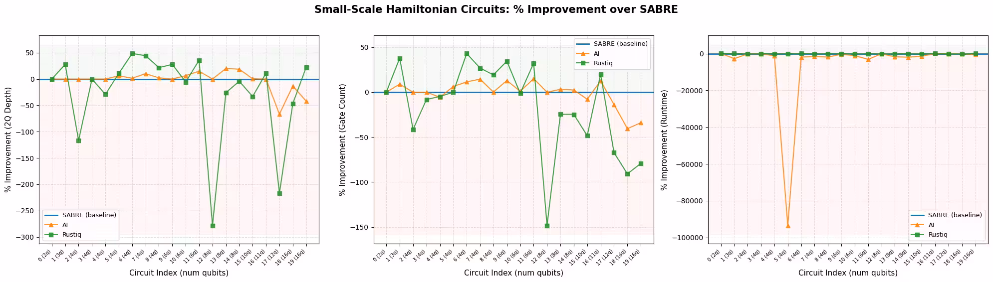
A esta escala, los tres gestores de pases funcionan bien y sus resultados promedio son cercanos entre sí. Esto se debe en gran medida a que los circuitos pequeños dejan poco margen para una mayor optimización, por lo que los métodos tienden a converger en soluciones similares.
En este ejemplo, Rustiq produce los resultados más variables, con los valores atípicos más grandes tanto en profundidad de dos qubits como en número de compuertas. Si bien esta variabilidad significa que a veces queda por detrás, también significa que Rustiq ocasionalmente encuentra mejores soluciones que los otros dos métodos. El transpilador de IA es más estable en sus resultados en comparación con SABRE y Rustiq, siguiendo de cerca la mayoría de los circuitos sin muchos valores atípicos.
En cuanto al tiempo de ejecución, SABRE y Rustiq son ambos rápidos, mientras que el transpilador potenciado por IA es notablemente más lento en ciertos circuitos.
Método con mejor rendimiento por métrica
El gráfico a continuación muestra con qué frecuencia cada método logró el mejor valor (más bajo) para cada métrica. Los empates son posibles: para los circuitos más simples, múltiples métodos pueden alcanzar la misma profundidad de dos qubits o número de compuertas óptimo. Cuando ocurre un empate, todos los métodos empatados reciben crédito, por lo que los porcentajes para una métrica dada pueden sumar más del 100%.
def plot_best_method_bars(results, metrics_list=None):
    """
    Plot a grouped bar chart showing the percentage of circuits
    where each method achieved the best (lowest) value for each metric.

    Ties are counted for all tied methods, so percentages per metric
    can sum to more than 100%.
    """
    if metrics_list is None:
        metrics_list = ["two_qubit_depth", "size", "runtime"]

    labels = {
        "two_qubit_depth": "2Q Depth",
        "size": "Gate Count",
        "runtime": "Runtime",
    }
    methods = _method_order(results)
    palette = {"SABRE": "#1f77b4", "AI": "#ff7f0e", "Rustiq": "#2ca02c"}

    by_index = {}
    for r in results:
        by_index.setdefault(r["qc_index"], []).append(r)
    n_circuits = len(by_index)

    win_data = {m: [] for m in methods}
    tie_counts = []
    metric_labels = []

    for metric in metrics_list:
        metric_labels.append(
            labels.get(metric, metric.replace("_", " ").title())
        )
        counts = Counter()
        ties = 0
        for group in by_index.values():
            min_val = min(r[metric] for r in group)
            best = [r["method"] for r in group if r[metric] == min_val]
            if len(best) > 1:
                ties += 1
            counts.update(best)
        tie_counts.append(ties)
        for m in methods:
            win_data[m].append(counts.get(m, 0) / n_circuits * 100)

    x = np.arange(len(metric_labels))
    width = 0.22
    fig, ax = plt.subplots(figsize=(8, 5))

    for i, method in enumerate(methods):
        bars = ax.bar(
            x + i * width,
            win_data[method],
            width,
            label=method,
            color=palette.get(method, None),
            edgecolor="black",
            linewidth=0.5,
        )
        for bar in bars:
            height = bar.get_height()
            if height > 0:
                ax.text(
                    bar.get_x() + bar.get_width() / 2,
                    height + 1.5,
                    f"{height:.0f}%",
                    ha="center",
                    va="bottom",
                    fontsize=9,
                )

    # Annotate tie counts below each metric label
    for j, ties in enumerate(tie_counts):
        if ties > 0:
            ax.text(
                x[j] + width,
                -8,
                f"({ties} tie{'s' if ties != 1 else ''})",
                ha="center",
                va="top",
                fontsize=8,
                color="gray",
            )

    ax.set_xticks(x + width)
    ax.set_xticklabels(metric_labels, fontsize=11)
    ax.set_ylabel("Circuits with best value (%)", fontsize=11)
    ax.set_title(
        "Best-Performing Method by Metric (ties counted for all tied methods)",
        fontsize=12,
        fontweight="bold",
    )
    ax.legend(frameon=True, fontsize=10)
    ax.set_ylim(-12, 120)
    ax.yaxis.set_major_formatter(ticker.PercentFormatter())
    ax.grid(axis="y", linestyle="--", alpha=0.4)

    plt.tight_layout()
    plt.show()
plot_best_method_bars(results_small)

En este ejemplo, los tres métodos tienen un rendimiento muy similar en los circuitos de pequeña escala. En profundidad de dos qubits y número de compuertas, la proporción de circuitos donde cada método es el mejor es parecida (aproximadamente 35–55%), y muchos circuitos terminan en empate porque los circuitos más simples a menudo tienen una única solución óptima que encuentran múltiples métodos. La diferencia más clara está en el tiempo de ejecución: SABRE y Rustiq son cada uno el más rápido en aproximadamente la mitad de los circuitos, mientras que el transpilador potenciado por IA raramente es el más veloz. Considerando las tres métricas en conjunto, Rustiq tiene una ligera ventaja general es el ganador más frecuente en profundidad de dos qubits y se mantiene competitivo en número de compuertas y tiempo de ejecución.
Paso 3: Ejecutar usando primitivas de Qiskit
Para evaluar cómo la calidad de la transpilación afecta la ejecución bajo ruido, usamos una técnica de circuito espejo. Para cada circuito transpilado , añadimos su inverso de modo que el circuito combinado es teóricamente la identidad. Comenzando desde el estado , una ejecución perfecta (sin ruido) devolvería la cadena de bits de todos ceros con probabilidad 1.
En la práctica, los errores de las compuertas se acumulan a lo largo del circuito, por lo que la probabilidad de recuperar disminuye. Un método de compilación que produce un circuito más superficial con menos compuertas acumulará menos ruido.
El enfoque del circuito espejo es atractivamente simple y escala a cualquier tamaño de circuito, ya que la salida esperada siempre es y no se requiere simulación clásica del estado ideal. Sin embargo, ten en cuenta las siguientes advertencias: el circuito espejo es una aproximación del circuito real (no el circuito en sí), duplica el número de compuertas (lo que exagera el efecto del ruido) y puede subestimar ciertos errores cuando el ruido se cancela simétricamente a través del límite del espejo.
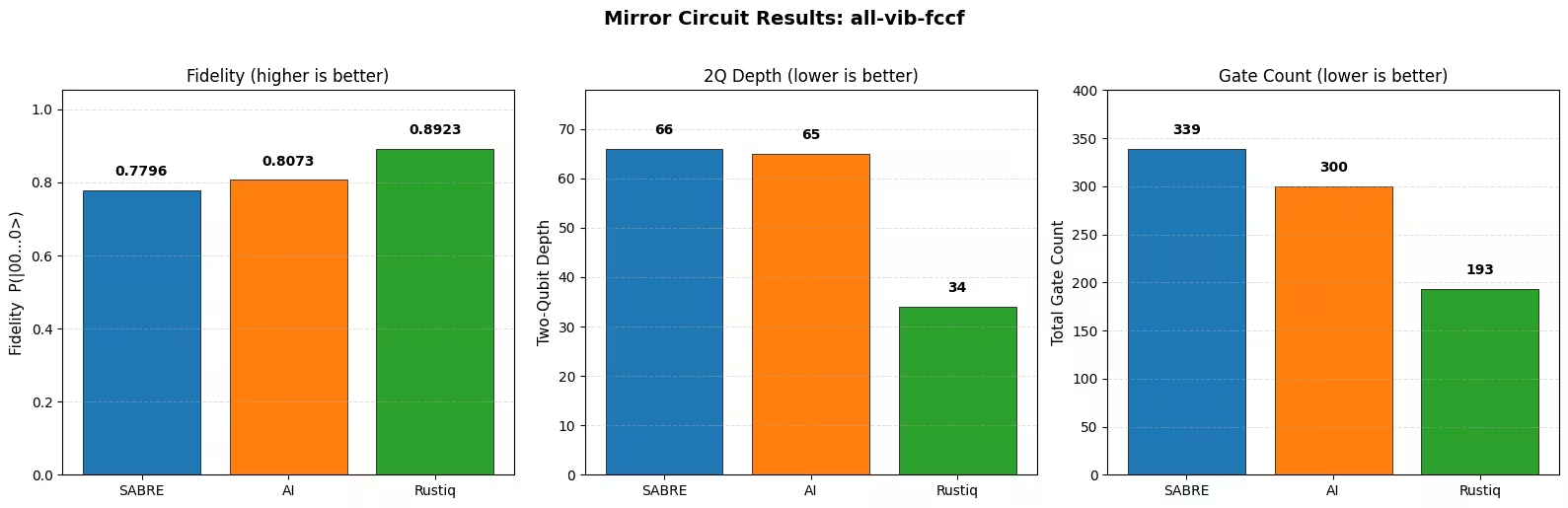
Seleccionamos el circuito con índice 6 del conjunto de pequeña escala y ejecutamos los circuitos espejo en un simulador Aer con un modelo de ruido depolarizante simple.
# Select circuit index 6 from the small-scale transpiled circuits
test_idx = 6
test_circuit = qc_small[test_idx]
print(f"Test circuit: {test_circuit.name}, {test_circuit.num_qubits} qubits")

# Get the transpiled versions
tqc_methods_small = {
    "SABRE": tqc_sabre_small[test_idx],
    "AI": tqc_ai_small[test_idx],
    "Rustiq": tqc_rustiq_small[test_idx],
}

# Show transpilation metrics for this circuit
print(f"\nTranspilation metrics for circuit index {test_idx}:")
for method, tqc in tqc_methods_small.items():
    depth_2q = tqc.depth(lambda x: x.operation.num_qubits == 2)
    size = tqc.size()
    print(f"  {method:8s}  2Q depth={depth_2q:5d}  size={size:6d}")
Test circuit: all-vib-fccf, 4 qubits

Transpilation metrics for circuit index 6:
  SABRE     2Q depth=   66  size=   339
  AI        2Q depth=   65  size=   300
  Rustiq    2Q depth=   34  size=   193
Construye los circuitos espejo (añade ), reasigna a índices de qubits contiguos para que el simulador maneje solo los qubits activos y ejecuta en un simulador Aer con ruido.
def remap_to_contiguous(tqc):
    """Remap a transpiled circuit to use contiguous qubit indices.

    Transpiled circuits target specific physical qubits (e.g., qubit 45, 67)
    on a large backend. This remaps them to 0, 1, 2, ... so Aer only
    simulates the active qubits.
    """
    active = sorted(
        {tqc.find_bit(q).index for inst in tqc.data for q in inst.qubits}
    )
    qubit_map = {old: new for new, old in enumerate(active)}
    new_qc = QuantumCircuit(len(active))
    for inst in tqc.data:
        old_indices = [tqc.find_bit(q).index for q in inst.qubits]
        new_qc.append(inst.operation, [qubit_map[i] for i in old_indices])
    return new_qc

def build_mirror_circuit(tqc):
    """Build a mirror circuit: U followed by U-dagger, with measurements.

    The combined circuit U-dagger @ U should be the identity, so measuring
    all zeros indicates a noise-free execution.
    """
    tqc_compact = remap_to_contiguous(tqc)
    mirror = tqc_compact.compose(tqc_compact.inverse())
    mirror.measure_all()
    return mirror

# Build a simple depolarizing noise model
noise_model = NoiseModel()
noise_model.add_all_qubit_quantum_error(
    depolarizing_error(0.001, 1),
    ["sx", "x", "rz"],  # ~0.1% per 1Q gate
)
noise_model.add_all_qubit_quantum_error(
    depolarizing_error(0.01, 2),
    ["cx", "ecr"],  # ~1% per 2Q gate
)

aer_sim = AerSimulator(noise_model=noise_model)

shots = 10000
fidelities = {}

for method, tqc in tqc_methods_small.items():
    mirror = build_mirror_circuit(tqc)

    sampler = SamplerV2(mode=aer_sim)
    job = sampler.run([mirror], shots=shots)
    result = job.result()
    counts = result[0].data.meas.get_counts()

    # Fidelity = fraction of all-zeros (error-free) outcomes
    n_qubits = mirror.num_qubits - mirror.num_clbits  # active qubits
    all_zeros = "0" * mirror.num_qubits
    fidelity = counts.get(all_zeros, 0) / shots
    fidelities[method] = fidelity
    print(
        f"{method:8s}  P(|00...0>) = {fidelity:.4f}  ({counts.get(all_zeros, 0)}/{shots})"
    )
SABRE     P(|00...0>) = 0.7796  (7796/10000)
AI        P(|00...0>) = 0.8073  (8073/10000)
Rustiq    P(|00...0>) = 0.8923  (8923/10000)
def plot_mirror_results(tqc_methods, fidelities, circuit_name):
    """
    Plot a three-panel comparison: fidelity, 2Q depth,
    and gate count for each compilation method.
    """
    methods = list(tqc_methods.keys())
    palette = {"SABRE": "#1f77b4", "AI": "#ff7f0e", "Rustiq": "#2ca02c"}
    colors = [palette.get(m, "gray") for m in methods]

    fidelity_vals = [fidelities[m] for m in methods]
    depth_vals = [
        tqc_methods[m].depth(lambda x: x.operation.num_qubits == 2)
        for m in methods
    ]
    size_vals = [tqc_methods[m].size() for m in methods]

    fig, axes = plt.subplots(1, 3, figsize=(16, 5))
    fig.suptitle(
        f"Mirror Circuit Results: {circuit_name}",
        fontsize=14,
        fontweight="bold",
        y=1.02,
    )

    def _annotate_bars(ax, bars, values, fmt="{}"):
        ymax = ax.get_ylim()[1]
        for bar, val in zip(bars, values):
            label = fmt.format(val)
            y = val + ymax * 0.03
            ax.text(
                bar.get_x() + bar.get_width() / 2,
                y,
                label,
                ha="center",
                va="bottom",
                fontsize=10,
                fontweight="bold",
            )

    # Panel 1: Survival Probability
    bars = axes[0].bar(
        methods, fidelity_vals, color=colors, edgecolor="black", linewidth=0.5
    )
    axes[0].set_ylabel("Fidelity  P(|00...0>)", fontsize=11)
    axes[0].set_title("Fidelity (higher is better)", fontsize=12)
    axes[0].set_ylim(
        0, max(fidelity_vals) * 1.18 if max(fidelity_vals) > 0 else 1.0
    )
    axes[0].grid(axis="y", linestyle="--", alpha=0.4)
    _annotate_bars(axes[0], bars, fidelity_vals, fmt="{:.4f}")

    # Panel 2: Two-Qubit Depth
    bars = axes[1].bar(
        methods, depth_vals, color=colors, edgecolor="black", linewidth=0.5
    )
    axes[1].set_ylabel("Two-Qubit Depth", fontsize=11)
    axes[1].set_title("2Q Depth (lower is better)", fontsize=12)
    axes[1].set_ylim(0, max(depth_vals) * 1.18)
    axes[1].grid(axis="y", linestyle="--", alpha=0.4)
    _annotate_bars(axes[1], bars, depth_vals)

    # Panel 3: Gate Count
    bars = axes[2].bar(
        methods, size_vals, color=colors, edgecolor="black", linewidth=0.5
    )
    axes[2].set_ylabel("Total Gate Count", fontsize=11)
    axes[2].set_title("Gate Count (lower is better)", fontsize=12)
    axes[2].set_ylim(0, max(size_vals) * 1.18)
    axes[2].grid(axis="y", linestyle="--", alpha=0.4)
    _annotate_bars(axes[2], bars, size_vals)

    plt.tight_layout()
    plt.show()

plot_mirror_results(tqc_methods_small, fidelities, test_circuit.name)
Observaciones
El método con la menor profundidad de dos qubits y el menor número de compuertas logra la mayor fidelidad, lo que es consistente con la expectativa de que los circuitos más cortos acumulan menos ruido. Incluso diferencias modestas en la profundidad y el número de compuertas se traducen en diferencias medibles en la fidelidad bajo el modelo de ruido depolarizante.
Ten en cuenta que estos resultados son para un único circuito. La clasificación relativa de los métodos puede cambiar de un circuito a otro dependiendo de la estructura del hamiltoniano.
Ejemplo de hardware a gran escala
En esta sección, comparamos los mismos tres métodos de compilación en circuitos hamiltonianos con 20 o más qubits. Estos circuitos son más representativos de las cargas de trabajo prácticas de simulación hamiltoniana y prueban cómo escala cada método en términos de calidad del circuito y tiempo de compilación.
Pasos 1-4 combinados
El flujo de trabajo sigue la misma estructura que el ejemplo de pequeña escala. Transpilamos todos los circuitos de gran escala con cada método, recopilamos métricas y enviamos un circuito espejo al hardware cuántico real.
results_large = []

tqc_sabre_large = capture_transpilation_metrics(
    results_large, pm_sabre, qc_large, "SABRE"
)
tqc_ai_large = capture_transpilation_metrics(
    results_large, pm_ai, qc_large, "AI"
)
tqc_rustiq_large = capture_transpilation_metrics(
    results_large, pm_rustiq, qc_large, "Rustiq"
)
[SABRE] Circuit 0 (all-vib-hc3h2cn): 2Q depth=2, size=258, time=0.16s
[SABRE] Circuit 1 (ham-graph-gnp_k-5): 2Q depth=345, size=4036, time=0.08s
[SABRE] Circuit 2 (TSP_Ncity-5): 2Q depth=187, size=2045, time=0.04s
[SABRE] Circuit 3 (tfim): 2Q depth=100, size=489, time=0.21s
[SABRE] Circuit 4 (all-vib-h2co): 2Q depth=30, size=570, time=0.18s
[SABRE] Circuit 5 (uuf100-ham): 2Q depth=414, size=4779, time=0.09s
[SABRE] Circuit 6 (uuf100-ham): 2Q depth=523, size=5667, time=0.11s
[SABRE] Circuit 7 (graph-gnp_k-4): 2Q depth=3028, size=24885, time=0.39s
[SABRE] Circuit 8 (uf100-ham): 2Q depth=700, size=8271, time=0.15s
[SABRE] Circuit 9 (uf100-ham): 2Q depth=698, size=8957, time=0.15s
[SABRE] Circuit 10 (TSP_Ncity-7): 2Q depth=432, size=6353, time=0.12s
[SABRE] Circuit 11 (all-vib-cyclo_propene): 2Q depth=30, size=1144, time=0.20s
[SABRE] Circuit 12 (TSP_Ncity-8): 2Q depth=704, size=10287, time=0.18s
[SABRE] Circuit 13 (uf100-ham): 2Q depth=2454, size=30195, time=0.46s
[SABRE] Circuit 14 (tfim): 2Q depth=245, size=3670, time=0.08s
[SABRE] Circuit 15 (flat100-ham): 2Q depth=154, size=3836, time=0.12s
[SABRE] Circuit 16 (graph-regular_reg-4): 2Q depth=863, size=14063, time=0.22s
[SABRE] Circuit 17 (tfim): 2Q depth=581, size=8810, time=0.15s
[SABRE] Circuit 18 (FH_D-1): 2Q depth=1704, size=9528, time=0.35s
[SABRE] Circuit 19 (TSP_Ncity-10): 2Q depth=1091, size=22041, time=0.38s
[SABRE] Circuit 20 (TSP_Ncity-10): 2Q depth=1091, size=22005, time=0.38s
[SABRE] Circuit 21 (ham-unary-color02-queen13_13_k-4): 2Q depth=224, size=8321, time=0.17s
[AI] Circuit 0 (all-vib-hc3h2cn): 2Q depth=2, size=258, time=0.17s
[AI] Circuit 1 (ham-graph-gnp_k-5): 2Q depth=323, size=4418, time=3.13s
[AI] Circuit 2 (TSP_Ncity-5): 2Q depth=161, size=2229, time=1.47s
[AI] Circuit 3 (tfim): 2Q depth=20, size=402, time=0.34s
[AI] Circuit 4 (all-vib-h2co): 2Q depth=38, size=661, time=0.19s
[AI] Circuit 5 (uuf100-ham): 2Q depth=391, size=5130, time=3.27s
[AI] Circuit 6 (uuf100-ham): 2Q depth=463, size=6095, time=4.23s
[AI] Circuit 7 (graph-gnp_k-4): 2Q depth=3207, size=25641, time=15.15s
[AI] Circuit 8 (uf100-ham): 2Q depth=637, size=8267, time=5.87s
[AI] Circuit 9 (uf100-ham): 2Q depth=632, size=9330, time=7.29s
[AI] Circuit 10 (TSP_Ncity-7): 2Q depth=452, size=7418, time=6.02s
[AI] Circuit 11 (all-vib-cyclo_propene): 2Q depth=38, size=1323, time=0.27s
[AI] Circuit 12 (TSP_Ncity-8): 2Q depth=609, size=11131, time=10.07s
[AI] Circuit 13 (uf100-ham): 2Q depth=2251, size=31128, time=38.77s
[AI] Circuit 14 (tfim): 2Q depth=165, size=3460, time=1.64s
[AI] Circuit 15 (flat100-ham): 2Q depth=91, size=3497, time=2.49s
[AI] Circuit 16 (graph-regular_reg-4): 2Q depth=664, size=15256, time=12.35s
[AI] Circuit 17 (tfim): 2Q depth=583, size=9157, time=6.28s
[AI] Circuit 18 (FH_D-1): 2Q depth=1193, size=7754, time=4.54s
[AI] Circuit 19 (TSP_Ncity-10): 2Q depth=1134, size=22577, time=25.64s
[AI] Circuit 20 (TSP_Ncity-10): 2Q depth=1172, size=23851, time=28.97s
[AI] Circuit 21 (ham-unary-color02-queen13_13_k-4): 2Q depth=219, size=8600, time=8.85s
[Rustiq] Circuit 0 (all-vib-hc3h2cn): 2Q depth=2, size=257, time=0.16s
[Rustiq] Circuit 1 (ham-graph-gnp_k-5): 2Q depth=640, size=5831, time=0.13s
[Rustiq] Circuit 2 (TSP_Ncity-5): 2Q depth=408, size=3985, time=0.08s
[Rustiq] Circuit 3 (tfim): 2Q depth=31, size=688, time=0.07s
[Rustiq] Circuit 4 (all-vib-h2co): 2Q depth=65, size=1058, time=2.91s
[Rustiq] Circuit 5 (uuf100-ham): 2Q depth=633, size=6757, time=0.14s
[Rustiq] Circuit 6 (uuf100-ham): 2Q depth=795, size=8495, time=0.17s
[Rustiq] Circuit 7 (graph-gnp_k-4): 2Q depth=13768, size=139793, time=2.92s
[Rustiq] Circuit 8 (uf100-ham): 2Q depth=1099, size=11878, time=0.25s
[Rustiq] Circuit 9 (uf100-ham): 2Q depth=911, size=11111, time=0.22s
[Rustiq] Circuit 10 (TSP_Ncity-7): 2Q depth=1183, size=13197, time=0.27s
[Rustiq] Circuit 11 (all-vib-cyclo_propene): 2Q depth=67, size=2491, time=13.56s
[Rustiq] Circuit 12 (TSP_Ncity-8): 2Q depth=1615, size=21358, time=0.48s
[Rustiq] Circuit 13 (uf100-ham): 2Q depth=2920, size=40465, time=0.91s
[Rustiq] Circuit 14 (tfim): 2Q depth=489, size=6552, time=0.15s
[Rustiq] Circuit 15 (flat100-ham): 2Q depth=378, size=5906, time=0.14s
[Rustiq] Circuit 16 (graph-regular_reg-4): 2Q depth=12163, size=168679, time=2.94s
[Rustiq] Circuit 17 (tfim): 2Q depth=1208, size=17042, time=0.36s
[Rustiq] Circuit 18 (FH_D-1): 2Q depth=1061, size=24000, time=0.47s
[Rustiq] Circuit 19 (TSP_Ncity-10): 2Q depth=2565, size=41340, time=1.38s
[Rustiq] Circuit 20 (TSP_Ncity-10): 2Q depth=2565, size=41275, time=1.38s
[Rustiq] Circuit 21 (ham-unary-color02-queen13_13_k-4): 2Q depth=808, size=17548, time=0.42s
print_summary_table(results_large)
Mean +/- std per compilation method
Method                2Q Depth              Gate Count             Runtime (s)
------------------------------------------------------------------------------
SABRE          709.1 +/- 783.8     9,100.5 +/- 8,493.1             0.2 +/- 0.1
AI             656.6 +/- 777.5     9,435.6 +/- 8,853.0            8.5 +/- 10.2
Rustiq     2,062.5 +/- 3,631.1   26,804.8 +/- 43,403.1             1.3 +/- 2.9

Mean % improvement vs SABRE (positive = better than SABRE)
Method                2Q Depth              Gate Count             Runtime (s)
------------------------------------------------------------------------------
AI             +9.6% +/- 22.8%          -3.4% +/- 9.4%    -3620.0% +/- 2405.5%
Rustiq      -154.5% +/- 273.9%      -137.1% +/- 233.2%     -527.0% +/- 1405.5%
print_per_circuit_comparison(results_large, num_rows=8)
2Q Depth (first 8 circuits by qubit count); * = best
Idx  Circuit            Q    SABRE       AI   Rustiq
----------------------------------------------------
  0  all-vib-hc3h2cn   24       2*       2*       2*
  1  ham-graph-gnp_k-  24      345     323*      640
  2  TSP_Ncity-5       25      187     161*      408
  3  tfim              26      100      20*       31
  4  all-vib-h2co      32      30*       38       65
  5  uuf100-ham        40      414     391*      633
  6  uuf100-ham        40      523     463*      795
  7  graph-gnp_k-4     40    3028*     3207    13768

Gate Count (first 8 circuits by qubit count); * = best
Idx  Circuit            Q    SABRE       AI   Rustiq
----------------------------------------------------
  0  all-vib-hc3h2cn   24      258      258     257*
  1  ham-graph-gnp_k-  24    4036*     4418     5831
  2  TSP_Ncity-5       25    2045*     2229     3985
  3  tfim              26      489     402*      688
  4  all-vib-h2co      32     570*      661     1058
  5  uuf100-ham        40    4779*     5130     6757
  6  uuf100-ham        40    5667*     6095     8495
  7  graph-gnp_k-4     40   24885*    25641   139793

Runtime (s) (first 8 circuits by qubit count); * = best
Idx  Circuit            Q    SABRE       AI   Rustiq
----------------------------------------------------
  0  all-vib-hc3h2cn   24     0.16     0.17    0.16*
  1  ham-graph-gnp_k-  24    0.08*     3.13     0.13
  2  TSP_Ncity-5       25    0.04*     1.47     0.08
  3  tfim              26     0.21     0.34    0.07*
  4  all-vib-h2co      32    0.18*     0.19     2.91
  5  uuf100-ham        40    0.09*     3.27     0.14
  6  uuf100-ham        40    0.11*     4.23     0.17
  7  graph-gnp_k-4     40    0.39*    15.15     2.92
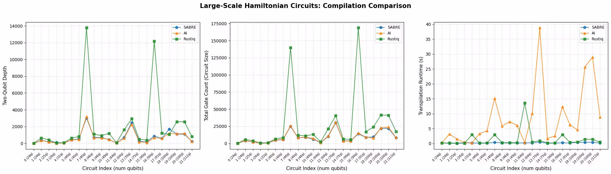
plot_transpilation_comparison(
    results_large,
    "Large-Scale Hamiltonian Circuits: Compilation Comparison",
)
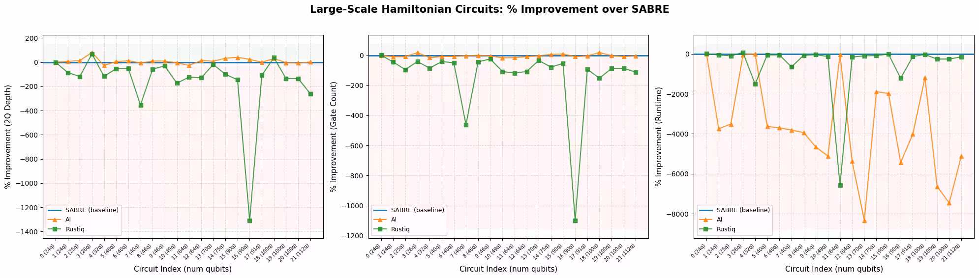
plot_pct_improvement_vs_sabre(
    results_large,
    "Large-Scale Hamiltonian Circuits",
)
plot_best_method_bars(results_large)

# Select circuit index 3 from the large-scale transpiled circuits
test_idx_large = 3
test_circuit_large = qc_large[test_idx_large]
print(
    f"Test circuit: {test_circuit_large.name}, {test_circuit_large.num_qubits} qubits"
)

tqc_methods_large = {
    "SABRE": tqc_sabre_large[test_idx_large],
    "AI": tqc_ai_large[test_idx_large],
    "Rustiq": tqc_rustiq_large[test_idx_large],
}

print(f"\nTranspilation metrics for circuit index {test_idx_large}:")
for method, tqc in tqc_methods_large.items():
    depth_2q = tqc.depth(lambda x: x.operation.num_qubits == 2)
    size = tqc.size()
    print(f"  {method:8s}  2Q depth={depth_2q:5d}  size={size:6d}")
Test circuit: tfim, 26 qubits

Transpilation metrics for circuit index 3:
  SABRE     2Q depth=  100  size=   489
  AI        2Q depth=   20  size=   402
  Rustiq    2Q depth=   31  size=   688
pm_mirror = generate_preset_pass_manager(
    optimization_level=0, backend=backend
)

for method, tqc in tqc_methods_large.items():
    # print the count ops for each circuit
    mirror = tqc.copy()
    mirror.compose(tqc.inverse(), inplace=True)
    mirror.measure_all()
    mirror = pm_mirror.run(mirror)
    print(f"\n{method} transpiled circuit:")
    print(tqc.count_ops())
    print(f"{method} mirror circuit count ops:")
    print(mirror.count_ops())
SABRE transpiled circuit:
OrderedDict({'sx': 211, 'rz': 163, 'cz': 104, 'x': 11})
SABRE mirror circuit count ops:
OrderedDict({'rz': 1170, 'sx': 422, 'cz': 208, 'measure': 156, 'x': 22, 'barrier': 1})

AI transpiled circuit:
OrderedDict({'sx': 165, 'rz': 162, 'cz': 68, 'x': 7})
AI mirror circuit count ops:
OrderedDict({'rz': 984, 'sx': 330, 'measure': 156, 'cz': 136, 'x': 14, 'barrier': 1})

Rustiq transpiled circuit:
OrderedDict({'sx': 316, 'rz': 225, 'cz': 140, 'x': 7})
Rustiq mirror circuit count ops:
OrderedDict({'rz': 1714, 'sx': 632, 'cz': 280, 'measure': 156, 'x': 14, 'barrier': 1})
# Build mirror circuits and submit to real hardware
# The inverse may introduce gates (e.g., sxdg) not in the backend's
# basis gate set, so we re-transpile the mirror circuit.
pm_mirror = generate_preset_pass_manager(
    optimization_level=0, backend=backend
)

shots_hw = 10000
hw_jobs = {}

for method, tqc in tqc_methods_large.items():
    mirror = tqc.copy()
    mirror.compose(tqc.inverse(), inplace=True)
    mirror.measure_all()

    # Re-transpile at opt level 0 to decompose into basis gates
    # without changing the layout or routing
    mirror = pm_mirror.run(mirror)

    sampler = SamplerV2(mode=backend)
    sampler.options.environment.job_tags = ["TUT_CMHSC"]
    job = sampler.run([mirror], shots=shots_hw)
    hw_jobs[method] = job
    print(f"{method}: submitted job {job.job_id()}")
SABRE: submitted job d8gvgq66983c73dqe5og
AI: submitted job d8gvgqe6983c73dqe5pg
Rustiq: submitted job d8gvgqm6983c73dqe5q0
# Retrieve results and compute fidelities
fidelities_large = {}

for method, job in hw_jobs.items():
    result = job.result()
    counts = result[0].data.meas.get_counts()

    n_qubits = backend.num_qubits
    all_zeros = "0" * n_qubits
    fidelity = counts.get(all_zeros, 0) / shots_hw
    fidelities_large[method] = fidelity
    print(
        f"{method:8s}  P(|00...0>) = {fidelity:.4f}  ({counts.get(all_zeros, 0)}/{shots_hw})"
    )
SABRE     P(|00...0>) = 0.0005  (5/10000)
AI        P(|00...0>) = 0.3267  (3267/10000)
Rustiq    P(|00...0>) = 0.1845  (1845/10000)
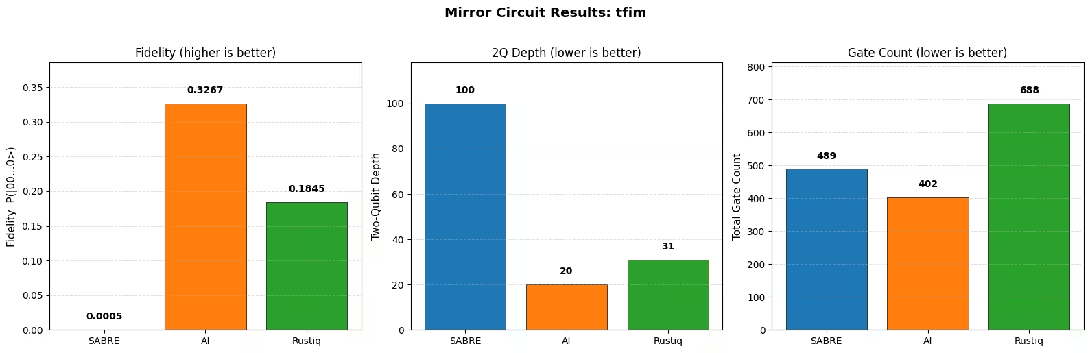
plot_mirror_results(
    tqc_methods_large, fidelities_large, test_circuit_large.name
)
Análisis de los resultados de compilación
Las comparaciones anteriores comparan SABRE, el transpilador potenciado por IA y Rustiq en circuitos de simulación hamiltoniana de la colección Hamlib tanto a pequeña como a gran escala.
Profundidad de dos qubits y número de compuertas
A gran escala, SABRE y el transpilador potenciado por IA son los dos mejores competidores, y cada uno lidera en una métrica diferente. Como muestra el gráfico de método con mejor rendimiento por métrica, SABRE produce el menor número de compuertas en la gran mayoría de los circuitos y es el método más rápido en casi todos ellos, lo que es consistente con una heurística diseñada para minimizar las compuertas SWAP insertadas y con las recientes optimizaciones de su distribución y enrutamiento. El transpilador potenciado por IA produce la menor profundidad de dos qubits en la mayoría de los circuitos, lo que es consistente con la parte de su objetivo de aprendizaje por refuerzo que apunta a la profundidad del circuito. La tabla resumen refleja la misma división: SABRE tiene el menor número promedio de compuertas, mientras que el transpilador de IA tiene la menor profundidad promedio de dos qubits. Ambos métodos son consistentes y confiables en toda la gama de circuitos.
Rustiq, diseñado específicamente para la síntesis de PauliEvolutionGate, produce el mejor resultado individual en solo una pequeña fracción de los circuitos de gran escala. Sus métricas promedio están fuertemente sesgadas por unos pocos valores atípicos significativos, visibles como grandes picos en el gráfico de comparación de compilación, donde Rustiq produce una profundidad y un número de compuertas sustancialmente mayores que los otros métodos. Sin estos valores atípicos, su rendimiento promedio estaría mucho más cerca de SABRE y el transpilador potenciado por IA.
La observación clave es que ningún método domina en todos los circuitos. Cada método supera a los otros en casos específicos, lo que hace que valga la pena probar todas las herramientas disponibles y seleccionar el mejor resultado para cada circuito.
Tiempo de ejecución
SABRE es consistentemente el método más rápido. Rustiq generalmente se ejecuta a una velocidad similar, pero puede producir valores atípicos donde la compilación tarda significativamente más. Esto es especialmente visible en los resultados de gran escala, donde algunos circuitos hacen que el tiempo de ejecución de Rustiq se dispare. Estos valores atípicos impactan fuertemente el tiempo de ejecución promedio, por lo que la mediana puede ser un resumen más representativo para Rustiq. El transpilador potenciado por IA es el más lento de los tres, con un tiempo de ejecución que crece notablemente en circuitos más grandes y complejos.
Resultados del circuito espejo
Los experimentos con circuitos espejo confirman la tendencia esperada: los métodos que producen menor profundidad de dos qubits y menos compuertas logran mayor fidelidad bajo ruido. Esto se cumple tanto en el simulador con ruido (pequeña escala) como en hardware real (gran escala).
Ten en cuenta que cada gráfico de circuito espejo refleja un único circuito, no el agregado. El ejemplo de hardware anterior usa un circuito tfim de 26 qubits, que resulta ser un caso donde SABRE produce una profundidad de dos qubits mucho mayor que el transpilador potenciado por IA y Rustiq, por lo que su fidelidad es correspondientemente mucho menor. Esto no es representativo de los resultados generales: en el conjunto completo de circuitos de gran escala, la profundidad de dos qubits de SABRE suele ser cercana a la del transpilador potenciado por IA, y los dos métodos cada uno lidera en métricas diferentes (el transpilador potenciado por IA en profundidad de dos qubits, SABRE en número de compuertas y tiempo de ejecución). Un único resultado de espejo prueba una versión duplicada de un circuito en lugar de la carga de trabajo completa, por lo que no debe interpretarse como un veredicto sobre la calidad general del método.
Recomendaciones
No existe una única mejor estrategia de transpilación para todos los circuitos. La mejor elección depende de la estructura del circuito, el objetivo de optimización y el presupuesto de tiempo de compilación disponible:
- SABRE es el valor predeterminado recomendado. Es rápido y confiable, y produce resultados sólidos en una amplia gama de circuitos. Para una mayor sintonía, los usuarios pueden aumentar los intentos de distribución y enrutamiento (consulta el tutorial de optimización con SABRE).
- El transpilador potenciado por IA vale la pena probarlo cuando el tiempo de compilación no es una restricción, especialmente cuando minimizar la profundidad de dos qubits es la prioridad: produjo la menor profundidad de dos qubits en la mayoría de los circuitos de gran escala en esta comparación.
- Rustiq está diseñado específicamente para circuitos con
PauliEvolutionGatey puede encontrar soluciones de muy baja profundidad y bajo número de compuertas, particularmente en circuitos más pequeños. En circuitos más grandes puede producir ocasionalmente resultados mucho mayores, por lo que es mejor usarlo como uno de varios métodos a probar en lugar de como valor predeterminado.
En la práctica, el mejor enfoque es ejecutar todos los métodos disponibles y elegir el mejor resultado para cada circuito. La sobrecarga de compilación de probar múltiples métodos es pequeña en comparación con la posible mejora en la calidad de ejecución en hardware real.
Próximos pasos
Si este tutorial te ha resultado útil, puede que te interese lo siguiente:
Referencias
[1] "LightSABRE: A Lightweight and Enhanced SABRE Algorithm". H. Zou, M. Treinish, K. Hartman, A. Ivrii, J. Lishman et al. https://arxiv.org/abs/2409.08368
[2] "Practical and efficient quantum circuit synthesis and transpiling with Reinforcement Learning". D. Kremer, V. Villar, H. Paik, I. Duran, I. Faro, J. Cruz-Benito et al. https://arxiv.org/abs/2405.13196
[3] "Pauli Network Circuit Synthesis with Reinforcement Learning". A. Dubal, D. Kremer, S. Martiel, V. Villar, D. Wang, J. Cruz-Benito et al. https://arxiv.org/abs/2503.14448
[4] "Faster and shorter synthesis of Hamiltonian simulation circuits". T. Goubault de Brugiere, S. Martiel et al. https://arxiv.org/abs/2404.03280