Experimento a escala de utilidad III

nota

Toshinari Itoko, Tamiya Onodera, Kifumi Numata (19 de julio de 2024)

Descarga el PDF de la conferencia original. Ten en cuenta que algunos fragmentos de código pueden quedar obsoletos, ya que son imágenes estáticas.

El tiempo aproximado de QPU para ejecutar este primer experimento es de 12 min 30 s. Hay un experimento adicional a continuación que requiere aproximadamente 4 min.

(Nota: es posible que este notebook no se evalúe en el tiempo permitido en el Plan Abierto. Asegúrate de usar los recursos de computación cuántica con prudencia.)

# Added by doQumentation — required packages for this notebook
!pip install -q numpy qiskit qiskit-ibm-runtime rustworkx

import qiskit

qiskit.__version__

'2.0.2'

import qiskit_ibm_runtime

qiskit_ibm_runtime.__version__

'0.40.1'

import numpy as np
import rustworkx as rx

from qiskit import QuantumCircuit
from qiskit.visualization import plot_histogram
from qiskit.visualization import plot_gate_map
from qiskit.transpiler.preset_passmanagers import generate_preset_pass_manager
from qiskit.providers import BackendV2
from qiskit.quantum_info import SparsePauliOp

from qiskit_ibm_runtime import QiskitRuntimeService
from qiskit_ibm_runtime import Sampler, Estimator, Batch, SamplerOptions

1. Introducción

Hagamos un repaso breve de los estados GHZ y del tipo de distribución que podrías esperar al aplicarles Sampler. Luego explicaremos con claridad el objetivo de esta lección.

1.1 Estado GHZ

El estado GHZ (estado de Greenberger-Horne-Zeilinger) para $n$ qubits se define como

$$\frac{1}{\sqrt 2}(|0\rangle ^ {\otimes n}+ |1\rangle^ {\otimes n})$$

De forma natural, se puede crear para 6 qubits con el siguiente circuito cuántico.

N = 6
qc = QuantumCircuit(N, N)

qc.h(0)
for i in range(N - 1):
    qc.cx(0, i + 1)

# qc.measure_all()
qc.barrier()
qc.measure(list(range(N)), list(range(N)))

qc.draw(output="mpl", idle_wires=False, scale=0.5)

print("Depth:", qc.depth())

Depth: 7

La profundidad no es demasiado grande, aunque ya sabes por lecciones anteriores que se puede mejorar. Elijamos un backend y transpilemos este circuito.

service = QiskitRuntimeService()
backend = service.least_busy(operational=True, simulator=False)
backend.name
# or
# backend = service.least_busy(operational=True)
# backend.name

'ibm_kingston'

pm = generate_preset_pass_manager(3, backend=backend)
qc_transpiled = pm.run(qc)
qc_transpiled.draw(output="mpl", idle_wires=False, fold=-1)

print("Depth:", qc_transpiled.depth())
print(
    "Two-qubit Depth:",
    qc_transpiled.depth(filter_function=lambda x: x.operation.num_qubits == 2),
)

Depth: 27
Two-qubit Depth: 11

De nuevo, la profundidad de dos qubits tras la transpilación no es demasiado grande. Pero para trabajar con un estado GHZ en más qubits, claramente necesitarás pensar en cómo optimizar el circuito. Ejecutemos esto con Sampler y veamos qué devuelve un ordenador cuántico real.

sampler = Sampler(mode=backend)
shots = 40000
job = sampler.run([qc_transpiled], shots=shots)
job_id = job.job_id()
print(job_id)

d147y20n2txg008jvv70

job.status()

'DONE'

job = service.job(job_id)
result = job.result()
plot_histogram(result[0].data.c.get_counts(), figsize=(30, 5))

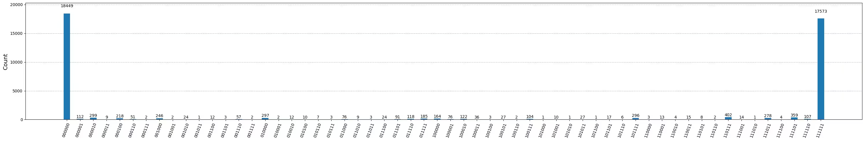
Este es el resultado del circuito GHZ de 6 qubits. Como puedes ver, los estados de todos los $|0\rangle$ y todos los $|1\rangle$ dominan, pero los errores son sustanciales. Intentemos ver qué tan grande puede ser un circuito GHZ en un dispositivo Eagle y aun así obtener resultados donde los estados correctos tengan al menos más del 50% de probabilidad.

1.2 Tu objetivo

Construye un circuito GHZ para 20 qubits o más de forma que, al medir, la fidelidad de tu estado GHZ sea > 0.5. Nota:

• Debes usar un dispositivo Eagle (min_num_qubits=127) y establecer el número de shots en 40 000.
• Debes ejecutar el circuito GHZ con la función execute_ghz_fidelity y calcular la fidelidad con la función check_ghz_fidelity_from_jobs.

Este ejercicio está pensado para que lo realices de forma independiente, aprovechando todo lo que has aprendido hasta ahora en este curso.

def execute_ghz_fidelity(
    ghz_circuit: QuantumCircuit,  # Quantum circuit to create GHZ state (Circuit after Routing or without Routing), Classical register name is "c"
    physical_qubits: list[int],  # Physical qubits to represent GHZ state
    backend: BackendV2,
    sampler_options: dict | SamplerOptions | None = None,
):
    N_SHOTS = 40_000
    N = len(physical_qubits)
    base_circuit = ghz_circuit.remove_final_measurements(inplace=False)
    # M_k measurement circuits
    mk_circuits = []
    for k in range(1, N + 1):
        circuit = base_circuit.copy()
        # change measurement basis
        for q in physical_qubits:
            circuit.rz(-k * np.pi / N, q)
            circuit.h(q)
        mk_circuits.append(circuit)

    obs = SparsePauliOp.from_sparse_list(
        [("Z" * N, physical_qubits, 1)], num_qubits=backend.num_qubits
    )
    job_ids = []
    pm1 = generate_preset_pass_manager(1, backend=backend)
    org_transpiled = pm1.run(ghz_circuit)
    mk_transpiled = pm1.run(mk_circuits)
    with Batch(backend=backend):
        sampler = Sampler(options=sampler_options)
        sampler.options.twirling.enable_measure = True
        job = sampler.run([org_transpiled], shots=N_SHOTS)
        job_ids.append(job.job_id())
        # print(f"Sampler job id: {job.job_id()}, shots={N_SHOTS}")
        estimator = Estimator()  # TREX is applied as default
        estimator.options.dynamical_decoupling.enable = True
        estimator.options.execution.rep_delay = 0.0005
        estimator.options.twirling.enable_measure = True
        job2 = estimator.run([(circ, obs) for circ in mk_transpiled], precision=1 / 100)
        job_ids.append(job2.job_id())
        # print("Estimator job id:", job2.job_id())
        return [job.job_id(), job2.job_id()]

def check_ghz_fidelity_from_jobs(
    sampler_job,
    estimator_job,
    num_qubits,
    shots=40_000,
):
    N = num_qubits
    sampler_result = sampler_job.result()
    counts = sampler_result[0].data.c.get_counts()
    all_zero = counts.get("0" * N, 0) / shots
    all_one = counts.get("1" * N, 0) / shots
    top3 = sorted(counts, key=counts.get, reverse=True)[:3]
    print(
        f"N={N}: |00..0>: {counts.get('0'*N, 0)}, |11..1>: {counts.get('1'*N, 0)}, |3rd>: {counts.get(top3[2], 0)} ({top3[2]})"
    )
    print(f"P(|00..0>)={all_zero}, P(|11..1>)={all_one}")

    estimator_result = estimator_job.result()
    non_diagonal = (1 / N) * sum(
        (-1) ** k * estimator_result[k - 1].data.evs for k in range(1, N + 1)
    )
    print(f"REM: Coherence (non-diagonal): {non_diagonal:.6f}")
    fidelity = 0.5 * (all_zero + all_one + non_diagonal)
    sigma = 0.5 * np.sqrt(
        (1 - all_zero - all_one) * (all_zero + all_one) / shots
        + sum(estimator_result[k].data.stds ** 2 for k in range(N)) / (N * N)
    )
    print(f"GHZ fidelity = {fidelity:.6f} ± {sigma:.6f}")
    if fidelity - 2 * sigma > 0.5:
        print("GME (genuinely multipartite entangled) test: Passed")
    else:
        print("GME (genuinely multipartite entangled) test: Failed")
    return {
        "fidelity": fidelity,
        "sigma": sigma,
        "shots": shots,
        "job_ids": [sampler_job.job_id(), estimator_job.job_id()],
    }

En este notebook aplicaremos tres estrategias para crear buenos estados GHZ usando 16 qubits y 30 qubits. Estos enfoques parten de las estrategias que ya conoces de lecciones anteriores.

2. Estrategia 1. Selección de qubits con conciencia del ruido

Primero especificamos un backend. Como trabajaremos extensamente con las propiedades de un backend específico, es buena idea especificar uno en concreto, en lugar de usar la opción least_busy.

backend = service.backend("ibm_strasbourg")  # eagle
twoq_gate = "ecr"
print(f"Device {backend.name} Loaded with {backend.num_qubits} qubits")
print(f"Two Qubit Gate: {twoq_gate}")

Device ibm_strasbourg Loaded with 127 qubits
Two Qubit Gate: ecr

Vamos a construir un circuito con muchas compuertas de dos qubits. Tiene sentido usar los qubits que presenten los menores errores al implementar esas compuertas de dos qubits. Encontrar la mejor "cadena de qubits" basándose en los errores de compuertas de 2 qubits reportados es un problema no trivial. Sin embargo, podemos definir algunas funciones para ayudarnos a determinar los mejores qubits a utilizar.

coupling_map = backend.target.build_coupling_map(twoq_gate)
G = coupling_map.graph

def to_edges(path):  # create edges list from node paths
    edges = []
    prev_node = None
    for node in path:
        if prev_node is not None:
            if G.has_edge(prev_node, node):
                edges.append((prev_node, node))
            else:
                edges.append((node, prev_node))
        prev_node = node
    return edges

def path_fidelity(path, correct_by_duration: bool = True, readout_scale: float = None):
    """Compute an estimate of the total fidelity of 2-qubit gates on a path.
    If `correct_by_duration` is true, each gate fidelity is worsen by
    scale = max_duration / duration, that is, gate_fidelity^scale.
    If `readout_scale` > 0 is supplied, readout_fidelity^readout_scale
    for each qubit on the path is multiplied to the total fielity.
    The path is given in node indices form, for example, [0, 1, 2].
    An external function `to_edges` is used to obtain edge list, for example, [(0, 1), (1, 2)]."""
    path_edges = to_edges(path)
    max_duration = max(backend.target[twoq_gate][qs].duration for qs in path_edges)

    def gate_fidelity(qpair):
        duration = backend.target[twoq_gate][qpair].duration
        scale = max_duration / duration if correct_by_duration else 1.0
        # 1.25 = (d+1)/d with d = 4
        return max(0.25, 1 - (1.25 * backend.target[twoq_gate][qpair].error)) ** scale

    def readout_fidelity(qubit):
        return max(0.25, 1 - backend.target["measure"][(qubit,)].error)

    total_fidelity = np.prod(
        [gate_fidelity(qs) for qs in path_edges]
    )  # two qubits gate fidelity for each path
    if readout_scale:
        total_fidelity *= (
            np.prod([readout_fidelity(q) for q in path]) ** readout_scale
        )  # multiply readout fidelity
    return total_fidelity

def flatten(paths, cutoff=None):  # cutoff is for not making run time too large
    return [
        path
        for s, s_paths in paths.items()
        for t, st_paths in s_paths.items()
        for path in st_paths[:cutoff]
        if s < t
    ]

N = 16  # Number of qubits to use in the GHZ circuit
num_qubits_in_chain = N

Usaremos las funciones anteriores para encontrar todos los caminos simples de N qubits entre todos los pares de nodos del grafo (Referencia: all_pairs_all_simple_paths).

Luego, usando la función path_fidelity creada anteriormente, encontraremos la mejor cadena de qubits, que es la que tiene la mayor fidelidad de camino.

from functools import partial

%%time
paths = rx.all_pairs_all_simple_paths(
    G.to_undirected(multigraph=False),
    min_depth=num_qubits_in_chain,
    cutoff=num_qubits_in_chain,
)
paths = flatten(paths, cutoff=25)  # If you have time, you could set a larger cutoff.
if not paths:
    raise Exception(
        f"No qubit chain with length={num_qubits_in_chain} exists in {backend.name}. Try smaller num_qubits_in_chain."
    )

print(f"Selecting the best from {len(paths)} candidate paths")

best_qubit_chain = max(
    paths, key=partial(path_fidelity, correct_by_duration=True, readout_scale=1.0)
)
assert len(best_qubit_chain) == num_qubits_in_chain
print(f"Predicted (best possible) process fidelity: {path_fidelity(best_qubit_chain)}")

Selecting the best from 6046 candidate paths
Predicted (best possible) process fidelity: 0.8929026784775056
CPU times: user 284 ms, sys: 10.9 ms, total: 295 ms
Wall time: 295 ms

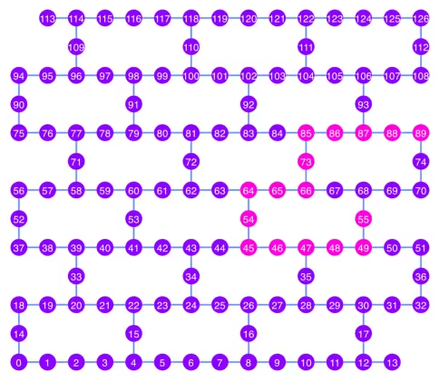
np.array(best_qubit_chain)

array([55, 49, 48, 47, 46, 45, 54, 64, 65, 66, 73, 85, 86, 87, 88, 89],
      dtype=uint64)

Grafiquemos la mejor cadena de qubits, mostrada en rosa, en el diagrama del mapa de acoplamiento.

qubit_color = []
for i in range(133):
    if i in best_qubit_chain:
        qubit_color.append("#ff00dd")  # pink
    else:
        qubit_color.append("#8c00ff")  # purple
plot_gate_map(
    backend, qubit_color=qubit_color, qubit_size=50, font_size=25, figsize=(6, 6)
)

2.1 Construir un circuito GHZ sobre la mejor cadena de qubits

Elegimos un qubit en el centro de la cadena para aplicarle primero la compuerta H. Esto debería reducir la profundidad del circuito aproximadamente a la mitad.

ghz1 = QuantumCircuit(max(best_qubit_chain) + 1, N)
ghz1.h(best_qubit_chain[N // 2])
for i in range(N // 2, 0, -1):
    ghz1.cx(best_qubit_chain[i], best_qubit_chain[i - 1])
for i in range(N // 2, N - 1, +1):
    ghz1.cx(best_qubit_chain[i], best_qubit_chain[i + 1])
ghz1.barrier()  # for visualization
ghz1.measure(best_qubit_chain, list(range(N)))
ghz1.draw(output="mpl", idle_wires=False, scale=0.5, fold=-1)

ghz1.depth()

10

pm = generate_preset_pass_manager(1, backend=backend)
ghz1_transpiled = pm.run(ghz1)
ghz1_transpiled.draw(output="mpl", idle_wires=False, fold=-1)

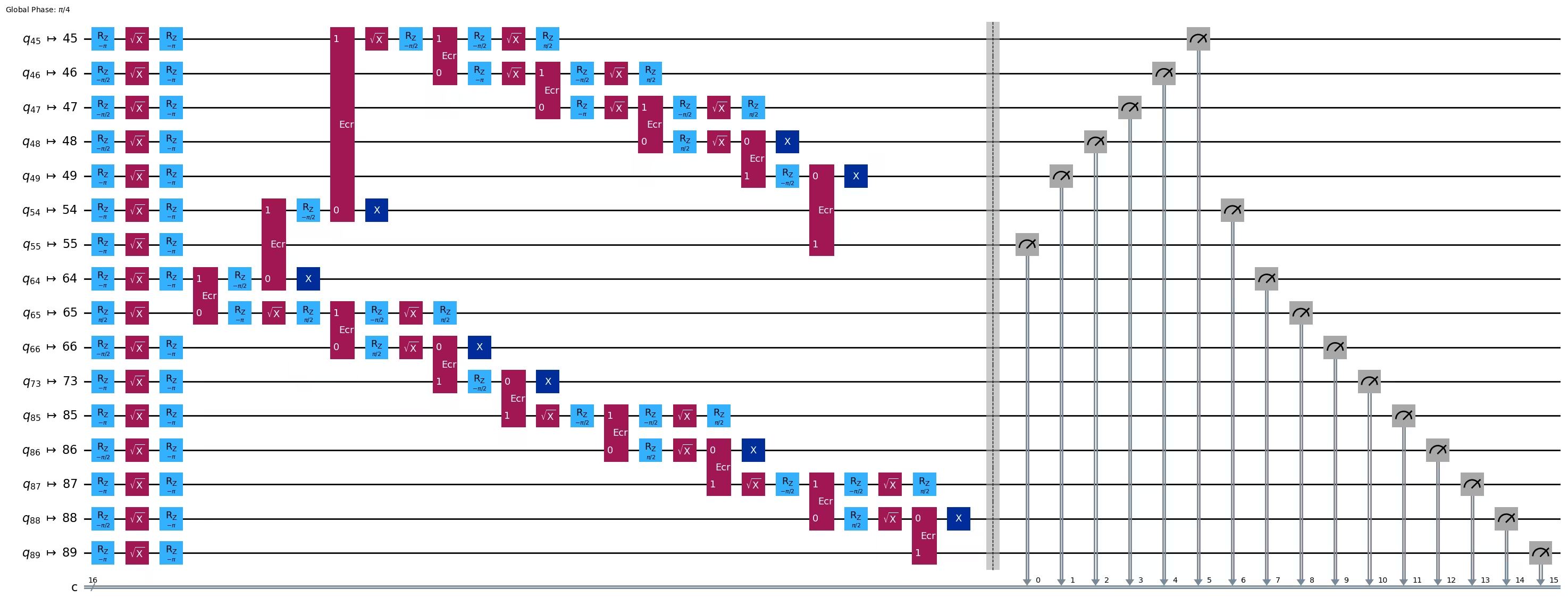
print("Depth:", ghz1_transpiled.depth())
print(
    "Two-qubit Depth:",
    ghz1_transpiled.depth(filter_function=lambda x: x.operation.num_qubits == 2),
)

Depth: 27
Two-qubit Depth: 8

opts = SamplerOptions()

res = execute_ghz_fidelity(
    ghz_circuit=ghz1,
    physical_qubits=best_qubit_chain,
    backend=backend,
    sampler_options=opts,
)

job_s = service.job(res[0])  # Use your job id showed above.
job_e = service.job(res[1])
print(job_s.status(), job_e.status())

DONE DONE

Ten cuidado de ejecutar la siguiente celda solo después de que los estados de los trabajos anteriores hayan pasado a 'DONE', para mostrar el resultado con la función check_ghz_fidelity_from_jobs.

N = 16
# Check fidelity from job IDs
res = check_ghz_fidelity_from_jobs(
    sampler_job=job_s,
    estimator_job=job_e,
    num_qubits=N,
)

N=16: |00..0>: 153, |11..1>: 8681, |3rd>: 2262 (1111111111101111)
P(|00..0>)=0.003825, P(|11..1>)=0.217025
REM: Coherence (non-diagonal): 0.073809
GHZ fidelity = 0.147329 ± 0.002438
GME (genuinely multipartite entangled) test: Failed

result = job_s.result()
plot_histogram(result[0].data.c.get_counts(), figsize=(30, 5))

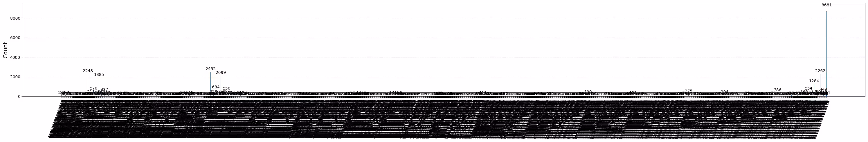
Este resultado no cumple los criterios. Pasemos a la siguiente idea.

3. Estrategia 2. Árbol balanceado de qubits

La siguiente idea es encontrar un árbol balanceado de qubits. Usando el árbol en lugar de la cadena, la profundidad del circuito debería ser menor. Antes de eso, eliminamos los nodos con errores de lectura "malos" y las aristas con errores de compuerta "malos" del grafo de acoplamiento.

BAD_READOUT_ERROR_THRESHOLD = 0.1
BAD_ECRGATE_ERROR_THRESHOLD = 0.1
bad_readout_qubits = [
    q
    for q in range(backend.num_qubits)
    if backend.target["measure"][(q,)].error > BAD_READOUT_ERROR_THRESHOLD
]
bad_ecrgate_edges = [
    qpair
    for qpair in backend.target["ecr"]
    if backend.target["ecr"][qpair].error > BAD_ECRGATE_ERROR_THRESHOLD
]
print("Bad readout qubits:", bad_readout_qubits)
print("Bad ECR gates:", bad_ecrgate_edges)

Bad readout qubits: [19, 28, 41, 72, 91, 114, 120]
Bad ECR gates: []

g = backend.coupling_map.graph.copy().to_undirected()
g.remove_edges_from(
    bad_ecrgate_edges
)  # remove edge first (otherwise might fail with a NoEdgeBetweenNodes error)
g.remove_nodes_from(bad_readout_qubits)

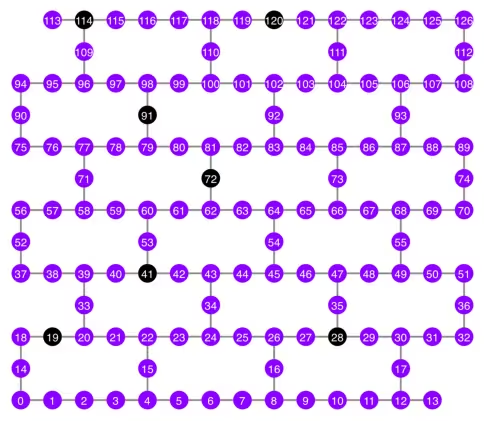
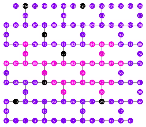
Grafiquemos el grafo del mapa de acoplamiento sin las aristas malas ni los qubits malos.

qubit_color = []
for i in range(133):
    if i in bad_readout_qubits:
        qubit_color.append("#000000")  # black
    else:
        qubit_color.append("#8c00ff")  # purple
line_color = []
for e in backend.target.build_coupling_map().get_edges():
    if e in bad_ecrgate_edges:
        line_color.append("#ffffff")  # white
    else:
        line_color.append("#888888")  # gray
plot_gate_map(
    backend,
    qubit_color=qubit_color,
    line_color=line_color,
    qubit_size=50,
    font_size=25,
    figsize=(6, 6),
)

Intentamos crear un estado GHZ de 16 qubits como antes.

N = 16

Llamamos a la función betweenness_centrality para encontrar un qubit que sirva de nodo raíz. El nodo con el valor más alto de centralidad de intermediación se encuentra en el centro del grafo. Referencia: https://www.rustworkx.org/tutorial/betweenness_centrality.html

O puedes seleccionarlo manualmente.

# central = 65 #Select the center node manually
c_degree = dict(rx.betweenness_centrality(g))
central = max(c_degree, key=c_degree.get)
central

66

Partiendo del nodo raíz, generamos un árbol mediante búsqueda en anchura (BFS). Referencia: https://qiskit.org/ecosystem/rustworkx/apiref/rustworkx.bfs_search.html#rustworkx-bfs-search

class TreeEdgesRecorder(rx.visit.BFSVisitor):
    def __init__(self, N):
        self.edges = []
        self.N = N

    def tree_edge(self, edge):
        self.edges.append(edge)
        if len(self.edges) >= self.N - 1:
            raise rx.visit.StopSearch()

vis = TreeEdgesRecorder(N)
rx.bfs_search(g, [central], vis)
best_qubits = sorted(list(set(q for e in vis.edges for q in (e[0], e[1]))))
# print('Tree edges:', vis.edges)

print("Qubits selected:", best_qubits)

Qubits selected: [54, 55, 63, 64, 65, 66, 67, 68, 69, 70, 73, 83, 84, 85, 86, 87]

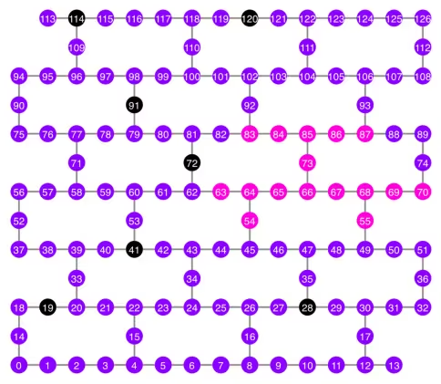
Grafiquemos los qubits seleccionados, mostrados en rosa, en el diagrama del mapa de acoplamiento.

qubit_color = []
for i in range(133):
    if i in bad_readout_qubits:
        qubit_color.append("#000000")  # black
    elif i in best_qubits:
        qubit_color.append("#ff00dd")  # pink
    else:
        qubit_color.append("#8c00ff")  # purple
plot_gate_map(
    backend,
    qubit_color=qubit_color,
    line_color=line_color,
    qubit_size=50,
    font_size=25,
    figsize=(6, 6),
)

Mostremos la estructura de árbol de los qubits.

from rustworkx.visualization import graphviz_draw

tree = rx.PyDiGraph()
tree.extend_from_weighted_edge_list(vis.edges)
tree.remove_nodes_from([n for n in range(max(best_qubits) + 1) if n not in best_qubits])

graphviz_draw(tree, method="dot")

ghz2 = QuantumCircuit(max(best_qubits) + 1, N)

ghz2.h(tree.edge_list()[0][0])  # apply H-gate to the root node
# Apply CNOT from the root node to the each edge.
for u, v in tree.edge_list():
    ghz2.cx(u, v)
ghz2.barrier()  # for visualization
ghz2.measure(best_qubits, list(range(N)))
ghz2.draw(output="mpl", idle_wires=False, scale=0.5)

ghz2.depth()

8

pm = generate_preset_pass_manager(1, backend=backend)
ghz2_transpiled = pm.run(ghz2)
ghz2_transpiled.draw(output="mpl", idle_wires=False, fold=-1)

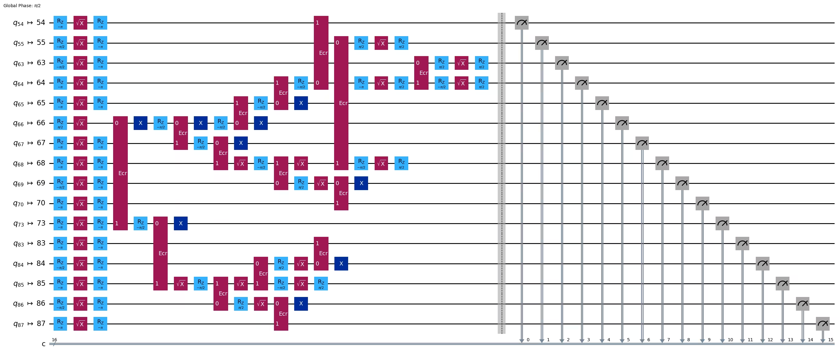
print("Depth:", ghz2_transpiled.depth())
print(
    "Two-qubit Depth:",
    ghz2_transpiled.depth(filter_function=lambda x: x.operation.num_qubits == 2),
)

Depth: 22
Two-qubit Depth: 6

La profundidad del circuito ahora es mucho menor que la de la estructura en cadena.

res = execute_ghz_fidelity(
    ghz_circuit=ghz2,
    physical_qubits=best_qubits,
    backend=backend,
    sampler_options=opts,
)

job_s = service.job(res[0])  # Use your job id showed above.
job_e = service.job(res[1])
print(job_s.status(), job_e.status())

DONE DONE

N = 16
# Check fidelity from job IDs
res = check_ghz_fidelity_from_jobs(
    sampler_job=job_s,
    estimator_job=job_e,
    num_qubits=N,
)

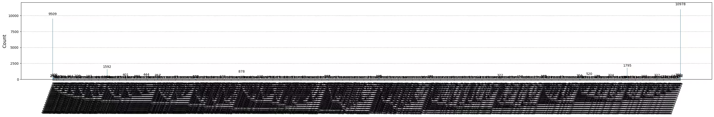
N=16: |00..0>: 9509, |11..1>: 10978, |3rd>: 1795 (1111110111111111)
P(|00..0>)=0.237725, P(|11..1>)=0.27445
REM: Coherence (non-diagonal): 0.606515
GHZ fidelity = 0.559345 ± 0.003188
GME (genuinely multipartite entangled) test: Passed

¡Hemos superado los criterios con éxito usando la estructura de árbol balanceado!

result = job_s.result()
plot_histogram(result[0].data.c.get_counts(), figsize=(30, 5))

Ahora intentemos crear un estado GHZ más grande: un estado GHZ de 30 qubits.

3.1 N = 30

Seguiremos el marco de Qiskit patterns.

• Paso 1: Mapear el problema a circuitos y operadores cuánticos
• Paso 2: Optimizar para el hardware objetivo
• Paso 3: Ejecutar en el hardware objetivo
• Paso 4: Postprocesar los resultados

Paso 1: Mapear el problema a circuitos y operadores cuánticos y Paso 2: Optimizar para el hardware objetivo

Aquí seleccionamos el nodo raíz manualmente.

central = 62  # Select the center node manually
# c_degree = dict(rx.betweenness_centrality(g))
# central = max(c_degree, key=c_degree.get)
# central

N = 30

vis = TreeEdgesRecorder(N)
rx.bfs_search(g, [central], vis)
best_qubits = sorted(list(set(q for e in vis.edges for q in (e[0], e[1]))))
print("Qubits selected:", best_qubits)

Qubits selected: [34, 35, 42, 43, 44, 45, 46, 47, 48, 53, 54, 56, 57, 58, 59, 60, 61, 62, 63, 64, 65, 66, 67, 68, 71, 73, 77, 84, 85, 86]

qubit_color = []
for i in range(133):
    if i in bad_readout_qubits:
        qubit_color.append("#000000")
    elif i in best_qubits:
        qubit_color.append("#ff00dd")
    else:
        qubit_color.append("#8c00ff")
line_color = []
for e in backend.target.build_coupling_map().get_edges():
    if e in bad_ecrgate_edges:
        line_color.append("#ffffff")
    else:
        line_color.append("#888888")
plot_gate_map(
    backend,
    qubit_color=qubit_color,
    line_color=line_color,
    qubit_size=50,
    font_size=25,
    figsize=(6, 6),
)

from rustworkx.visualization import graphviz_draw

tree = rx.PyDiGraph()
tree.extend_from_weighted_edge_list(vis.edges)
tree.remove_nodes_from([n for n in range(max(best_qubits) + 1) if n not in best_qubits])

graphviz_draw(tree, method="dot")

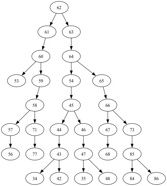
La profundidad de este árbol es 5.

ghz3 = QuantumCircuit(max(best_qubits) + 1, N)

ghz3.h(tree.edge_list()[0][0])  # apply H-gate to the root node
# Apply CNOT from the root node to the each edge.
for u, v in tree.edge_list():
    ghz3.cx(u, v)
ghz3.barrier()  # for visualization
ghz3.measure(best_qubits, list(range(N)))
ghz3.draw(output="mpl", idle_wires=False, fold=-1)

ghz3.depth()

11

pm = generate_preset_pass_manager(1, backend=backend)
ghz3_transpiled = pm.run(ghz3)
ghz3_transpiled.draw(output="mpl", idle_wires=False, fold=-1)

print("Depth:", ghz3_transpiled.depth())
print(
    "Two-qubit Depth:",
    ghz3_transpiled.depth(filter_function=lambda x: x.operation.num_qubits == 2),
)

Depth: 31
Two-qubit Depth: 9

3.2 Seleccionar un nodo raíz diferente manualmente

central = 54

vis = TreeEdgesRecorder(N)
rx.bfs_search(g, [central], vis)
best_qubits = sorted(list(set(q for e in vis.edges for q in (e[0], e[1]))))
print("Qubits selected:", best_qubits)

Qubits selected: [23, 24, 25, 34, 35, 42, 43, 44, 45, 46, 47, 48, 49, 50, 54, 55, 60, 61, 62, 63, 64, 65, 66, 67, 68, 69, 73, 84, 85, 86]

from rustworkx.visualization import graphviz_draw

tree = rx.PyDiGraph()
tree.extend_from_weighted_edge_list(vis.edges)
tree.remove_nodes_from([n for n in range(max(best_qubits) + 1) if n not in best_qubits])

graphviz_draw(tree, method="dot")

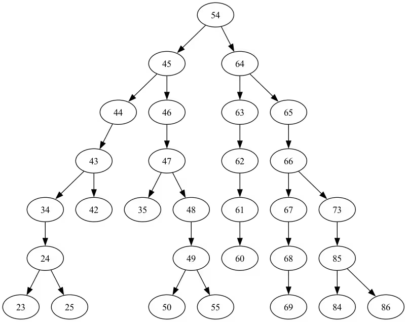
La profundidad de este árbol es 6.

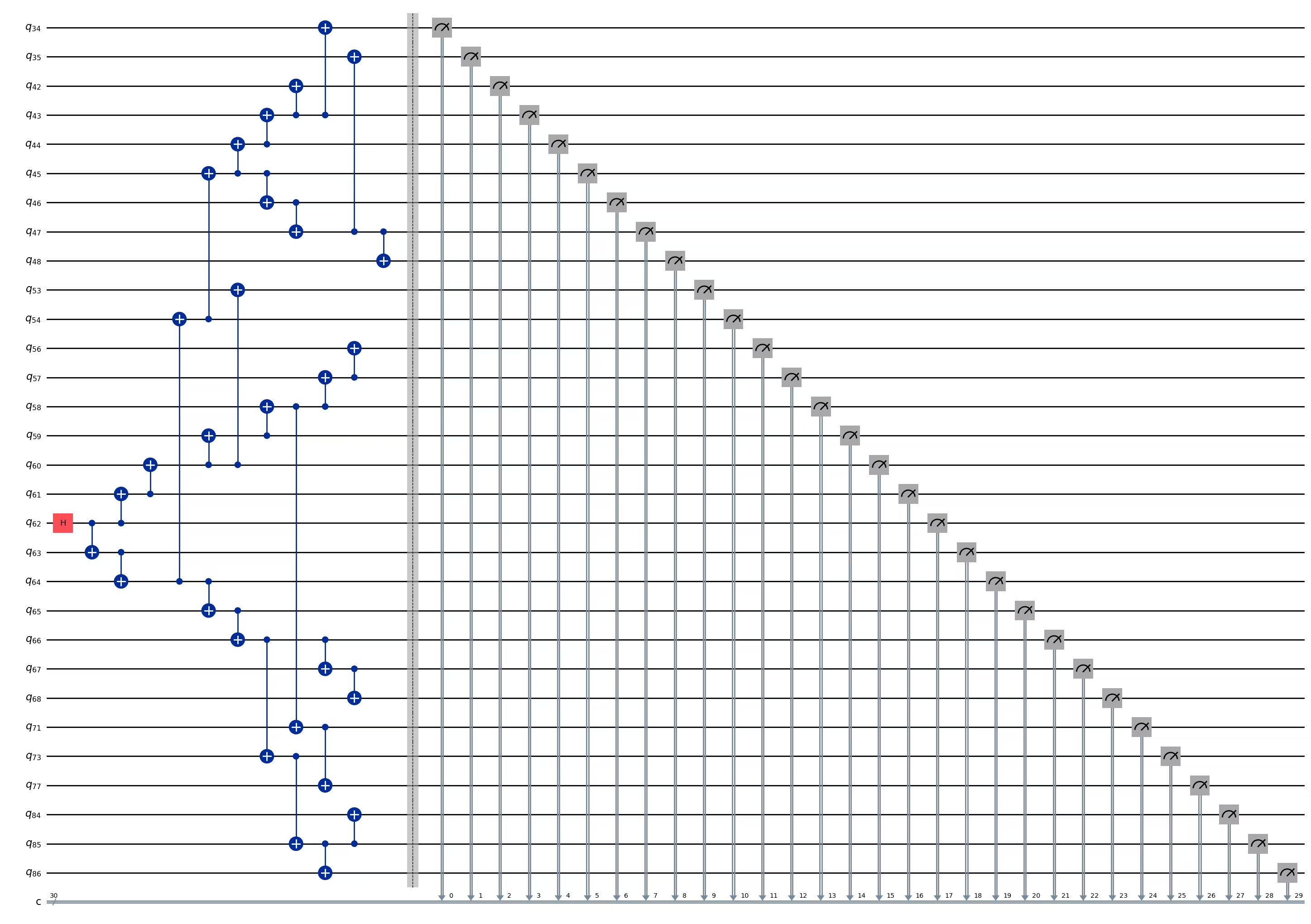
ghz3 = QuantumCircuit(max(best_qubits) + 1, N)

ghz3.h(tree.edge_list()[0][0])  # apply H-gate to the root node
# Apply CNOT from the root node to the each edge.
for u, v in tree.edge_list():
    ghz3.cx(u, v)
ghz3.barrier()  # for visualization
ghz3.measure(best_qubits, list(range(N)))
ghz3.draw(output="mpl", idle_wires=False, fold=-1)

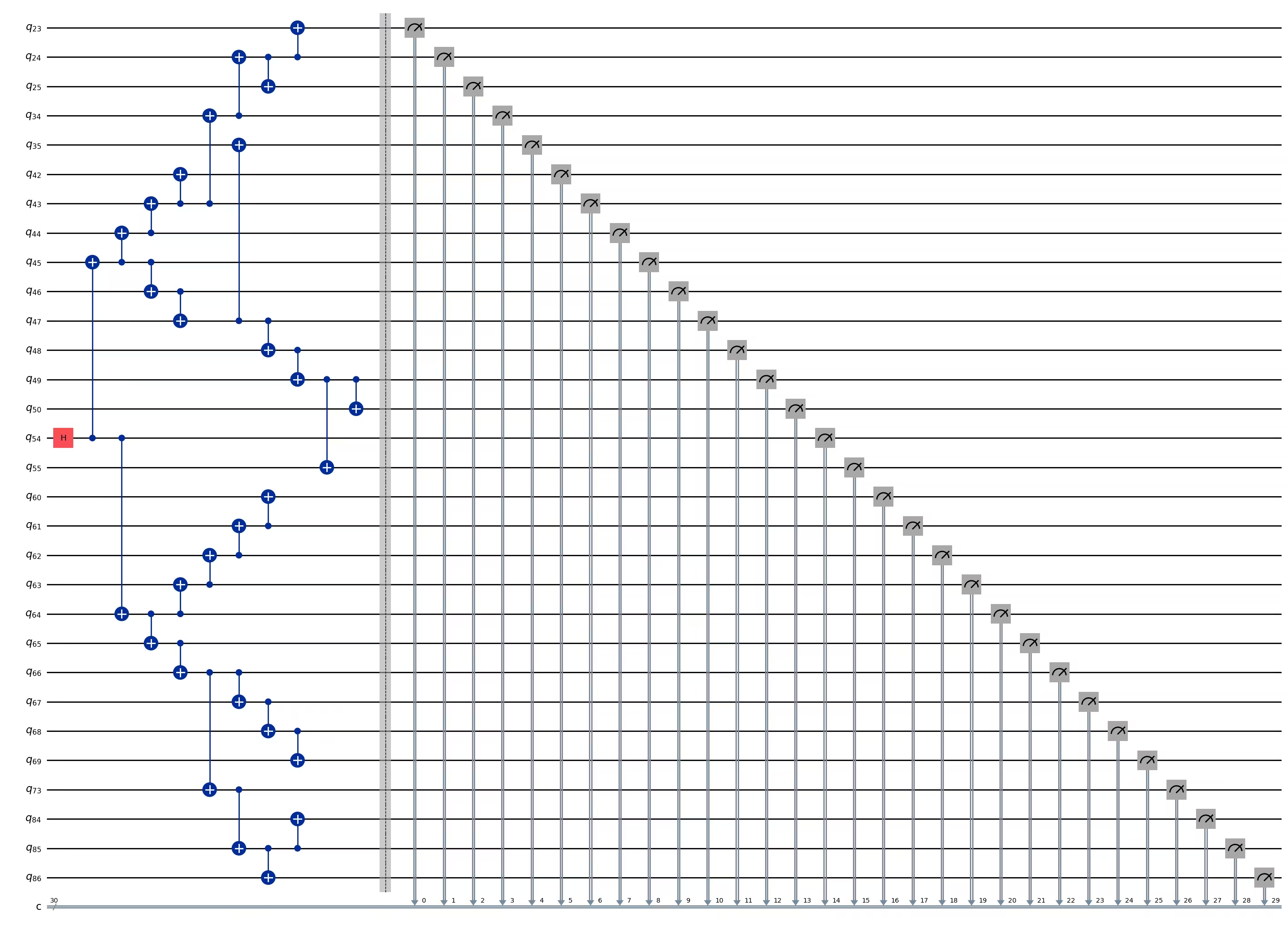
ghz3.depth()

11

pm = generate_preset_pass_manager(1, backend=backend)
ghz3_transpiled = pm.run(ghz3)
ghz3_transpiled.draw(output="mpl", idle_wires=False, fold=-1)

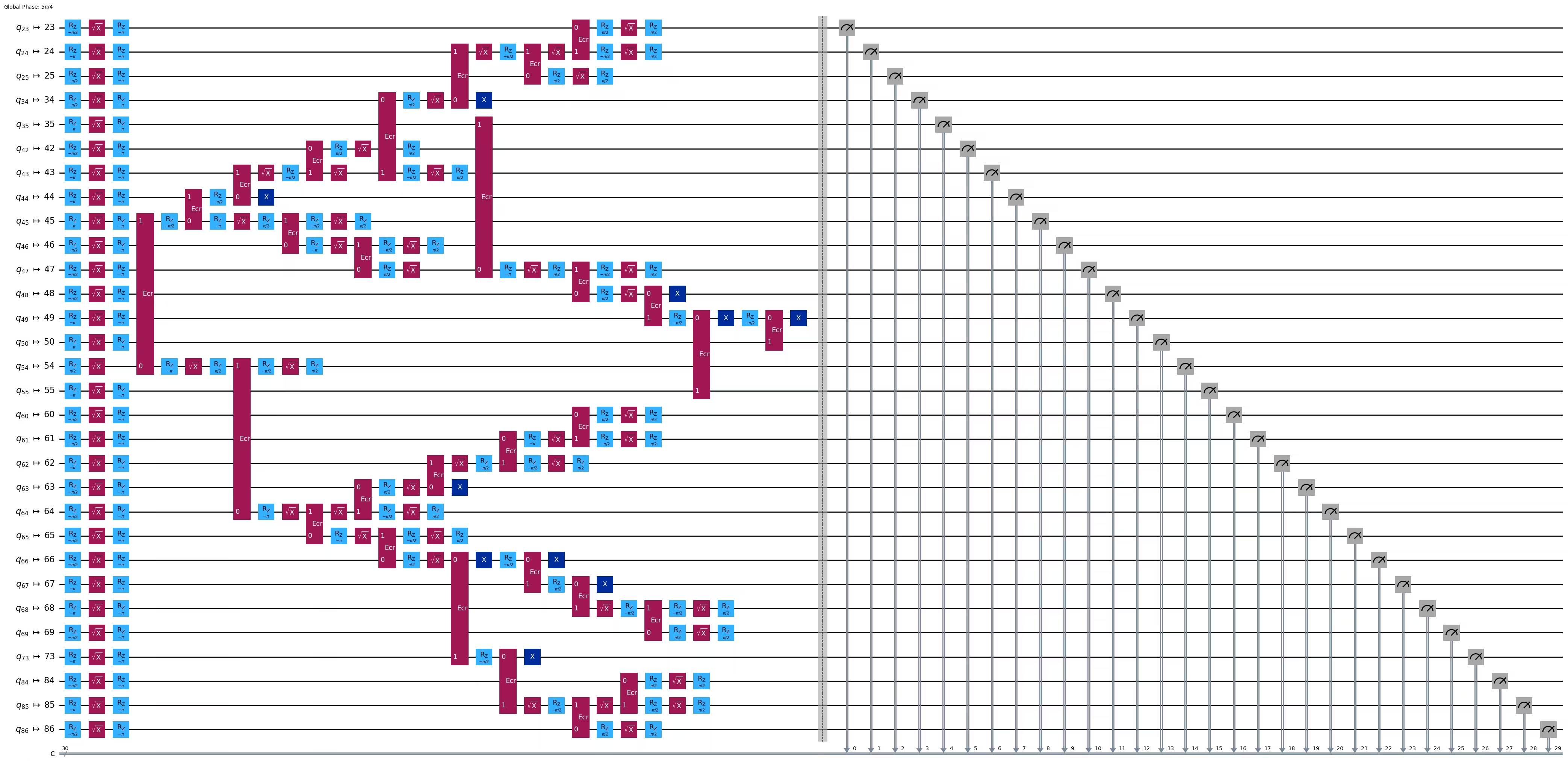
print("Depth:", ghz3_transpiled.depth())
print(
    "Two-qubit Depth:",
    ghz3_transpiled.depth(filter_function=lambda x: x.operation.num_qubits == 2),
)

Depth: 30
Two-qubit Depth: 9

Sorprendentemente, aunque la profundidad del árbol aumentó de 5 a 6, ¡la profundidad de dos qubits disminuyó de 9 a 8! Así que usemos el último circuito.

Paso 3: Ejecutar en el hardware objetivo

res = execute_ghz_fidelity(
    ghz_circuit=ghz3,
    physical_qubits=best_qubits,
    backend=backend,
    sampler_options=opts,
)

job_s = service.job(res[0])  # Use your job id showed above.
job_e = service.job(res[1])
print(job_s.status(), job_e.status())

DONE DONE

Paso 4: Postprocesar los resultados

N = 30
# Check fidelity from job IDs
res = check_ghz_fidelity_from_jobs(
    sampler_job=job_s,
    estimator_job=job_e,
    num_qubits=N,
)

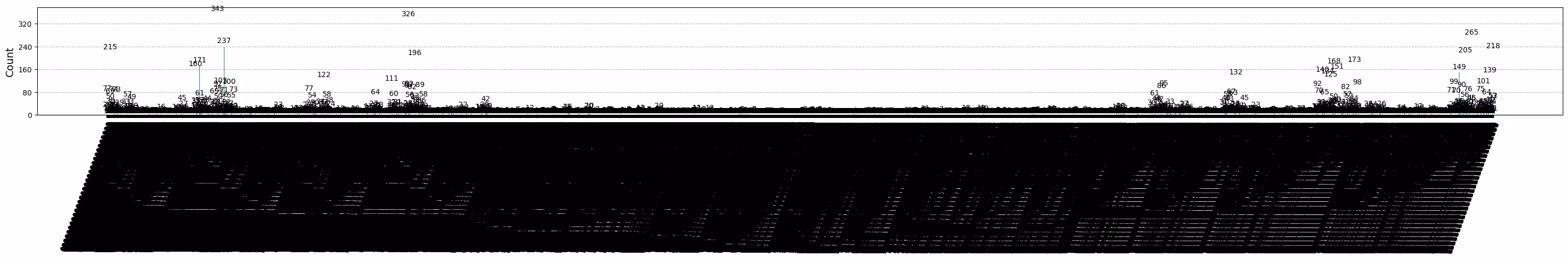
N=30: |00..0>: 4, |11..1>: 218, |3rd>: 265 (111111111111111011111111111111)
P(|00..0>)=0.0001, P(|11..1>)=0.00545
REM: Coherence (non-diagonal): 0.187073
GHZ fidelity = 0.096312 ± 0.003254
GME (genuinely multipartite entangled) test: Failed

Como puedes ver, este resultado no cumple los criterios.

# It will take some time
result = job_s.result()
plot_histogram(result[0].data.c.get_counts(), figsize=(30, 5))

4. Estrategia 3. Ejecutar con las opciones de supresión de errores

Puedes configurar las opciones de supresión de errores en Sampler V2. Consulta la guía Configurar la mitigación de errores y la referencia de la API ExecutionOptionsV2 para más información.

opts = SamplerOptions()
opts.dynamical_decoupling.enable = True
opts.execution.rep_delay = 0.0005
opts.twirling.enable_gates = True

res = execute_ghz_fidelity(
    ghz_circuit=ghz3,
    physical_qubits=best_qubits,
    backend=backend,
    sampler_options=opts,
)

job_s = service.job(res[0])  # Use your job id showed above.
job_e = service.job(res[1])
print(job_s.status(), job_e.status())

DONE DONE

N = 30

# Check fidelity from job IDs
res = check_ghz_fidelity_from_jobs(
    sampler_job=job_s,
    estimator_job=job_e,
    num_qubits=N,
)

N=30: |00..0>: 1459, |11..1>: 1543, |3rd>: 359 (111111111111111111111111111110)
P(|00..0>)=0.036475, P(|11..1>)=0.038575
REM: Coherence (non-diagonal): 0.165532
GHZ fidelity = 0.120291 ± 0.003369
GME (genuinely multipartite entangled) test: Failed

# It will take some time
result = job_s.result()
plot_histogram(result[0].data.c.get_counts(), figsize=(30, 5))

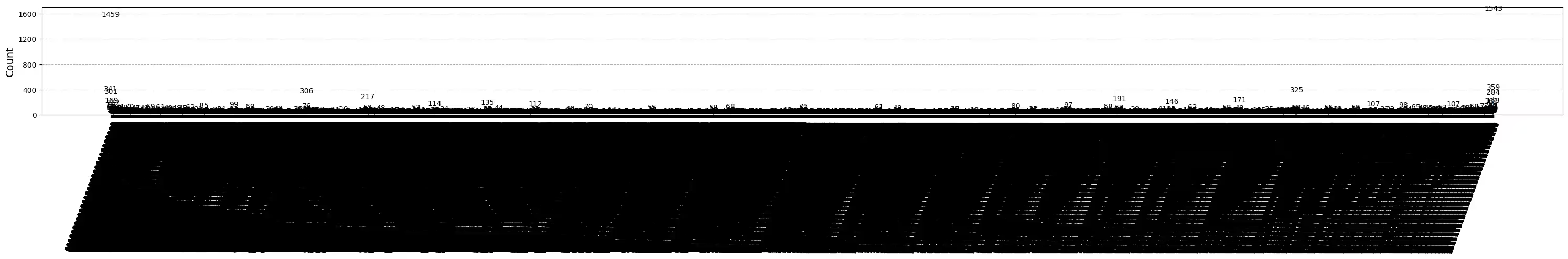
El resultado ha mejorado, pero aún no cumple los criterios.

Hemos visto tres ideas hasta ahora. Puedes combinar y ampliar estas ideas, o proponer las tuyas propias para crear un circuito GHZ mejor. Ahora revisemos el objetivo nuevamente.

5. Tu objetivo (recapitulación)

Construye un circuito GHZ para 20 qubits o más de modo que el resultado de la medición cumpla los criterios: la fidelidad de tu estado GHZ debe ser > 0,5.

• Debes usar un dispositivo Eagle (como ibm_brisbane) y establecer el número de disparos en 40.000.
• Debes ejecutar el circuito GHZ usando la función execute_ghz_fidelity y calcular la fidelidad con la función check_ghz_fidelity_from_jobs. Necesitas encontrar el mayor número de qubits — circuito GHZ que cumpla los criterios. Escribe tu código a continuación y muestra el resultado con la función check_ghz_fidelity_from_jobs.

Ahora implementamos el mismo flujo de trabajo GHZ que en el material anterior, pero en un dispositivo Heron. Esto te brinda experiencia con el diseño y las características de los procesadores Heron. No se introducen nuevas estrategias.

El tiempo aproximado de QPU para ejecutar este siguiente experimento es de 4 min 40 s.

service = QiskitRuntimeService()
backend = service.backend("ibm_kingston")
# backend = service.backend("ibm_fez")

twoq_gate = "cz"
print(f"Device {backend.name} Loaded with {backend.num_qubits} qubits")
print(f"Two Qubit Gate: {twoq_gate}")

Device ibm_kingston Loaded with 156 qubits
Two Qubit Gate: cz

BAD_READOUT_ERROR_THRESHOLD = 0.1
BAD_CZGATE_ERROR_THRESHOLD = 0.1
bad_readout_qubits = [
    q
    for q in range(backend.num_qubits)
    if backend.target["measure"][(q,)].error > BAD_READOUT_ERROR_THRESHOLD
]
bad_czgate_edges = [
    qpair
    for qpair in backend.target["cz"]
    if backend.target["cz"][qpair].error > BAD_CZGATE_ERROR_THRESHOLD
]
print("Bad readout qubits:", bad_readout_qubits)
print("Bad CZ gates:", bad_czgate_edges)

Bad readout qubits: [112, 113, 120, 131, 146]
Bad CZ gates: [(111, 112), (112, 111), (112, 113), (113, 112), (120, 121), (121, 120), (130, 131), (131, 130), (145, 146), (146, 145), (146, 147), (147, 146)]

g = backend.coupling_map.graph.copy().to_undirected()
g.remove_edges_from(
    bad_czgate_edges
)  # remove edge first (otherwise might fail with a NoEdgeBetweenNodes error)
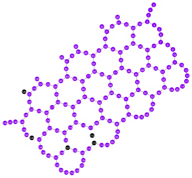
g.remove_nodes_from(bad_readout_qubits)

qubit_color = []
for i in range(backend.num_qubits):
    if i in bad_readout_qubits:
        qubit_color.append("#000000")  # black
    else:
        qubit_color.append("#8c00ff")  # purple
line_color = []
for e in backend.target.build_coupling_map().get_edges():
    if e in bad_czgate_edges:
        line_color.append("#ffffff")  # white
    else:
        line_color.append("#888888")  # gray
plot_gate_map(
    backend,
    qubit_color=qubit_color,
    line_color=line_color,
    qubit_size=60,
    font_size=30,
    figsize=(10, 10),
)

N = 40
central = 100  # Select the center node manually
# c_degree = dict(rx.betweenness_centrality(g))
# central = max(c_degree, key=c_degree.get)
# central

class TreeEdgesRecorder(rx.visit.BFSVisitor):
    def __init__(self, N):
        self.edges = []
        self.N = N

    def tree_edge(self, edge):
        self.edges.append(edge)
        if len(self.edges) >= self.N - 1:
            raise rx.visit.StopSearch()

vis = TreeEdgesRecorder(N)
rx.bfs_search(g, [central], vis)
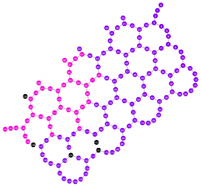
best_qubits = sorted(list(set(q for e in vis.edges for q in (e[0], e[1]))))
print("Qubits selected:", best_qubits)

Qubits selected: [61, 65, 76, 77, 80, 81, 82, 83, 84, 85, 86, 87, 96, 97, 100, 101, 102, 103, 104, 105, 106, 107, 108, 109, 116, 117, 121, 122, 123, 124, 125, 126, 127, 136, 140, 141, 142, 143, 144, 145]

qubit_color = []
for i in range(backend.num_qubits):
    if i in bad_readout_qubits:
        qubit_color.append("#000000")
    elif i in best_qubits:
        qubit_color.append("#ff00dd")
    else:
        qubit_color.append("#8c00ff")
line_color = []
for e in backend.target.build_coupling_map().get_edges():
    if e in bad_czgate_edges:
        line_color.append("#ffffff")
    else:
        line_color.append("#888888")
plot_gate_map(
    backend,
    qubit_color=qubit_color,
    line_color=line_color,
    qubit_size=60,
    font_size=30,
    figsize=(10, 10),
)

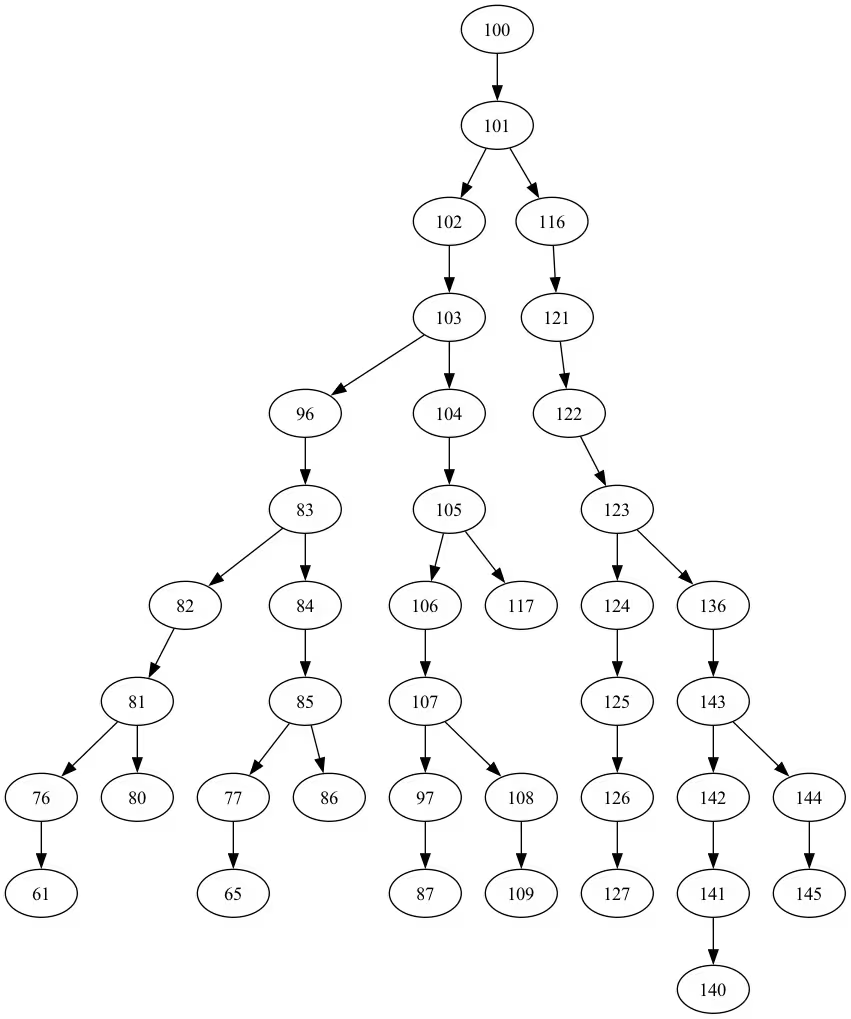
from rustworkx.visualization import graphviz_draw

tree = rx.PyDiGraph()
tree.extend_from_weighted_edge_list(vis.edges)
tree.remove_nodes_from([n for n in range(max(best_qubits) + 1) if n not in best_qubits])

graphviz_draw(tree, method="dot")

ghz_h = QuantumCircuit(max(best_qubits) + 1, N)

ghz_h.h(tree.edge_list()[0][0])  # apply H-gate to the root node
# Apply CNOT from the root node to the each edge.
for u, v in tree.edge_list():
    ghz_h.cx(u, v)
ghz_h.barrier()  # for visualization
ghz_h.measure(best_qubits, list(range(N)))
ghz_h.draw(output="mpl", idle_wires=False, fold=-1)

ghz_h.depth()

15

pm = generate_preset_pass_manager(1, backend=backend)
ghz_h_transpiled = pm.run(ghz_h)
ghz_h_transpiled.draw(output="mpl", idle_wires=False, fold=-1)

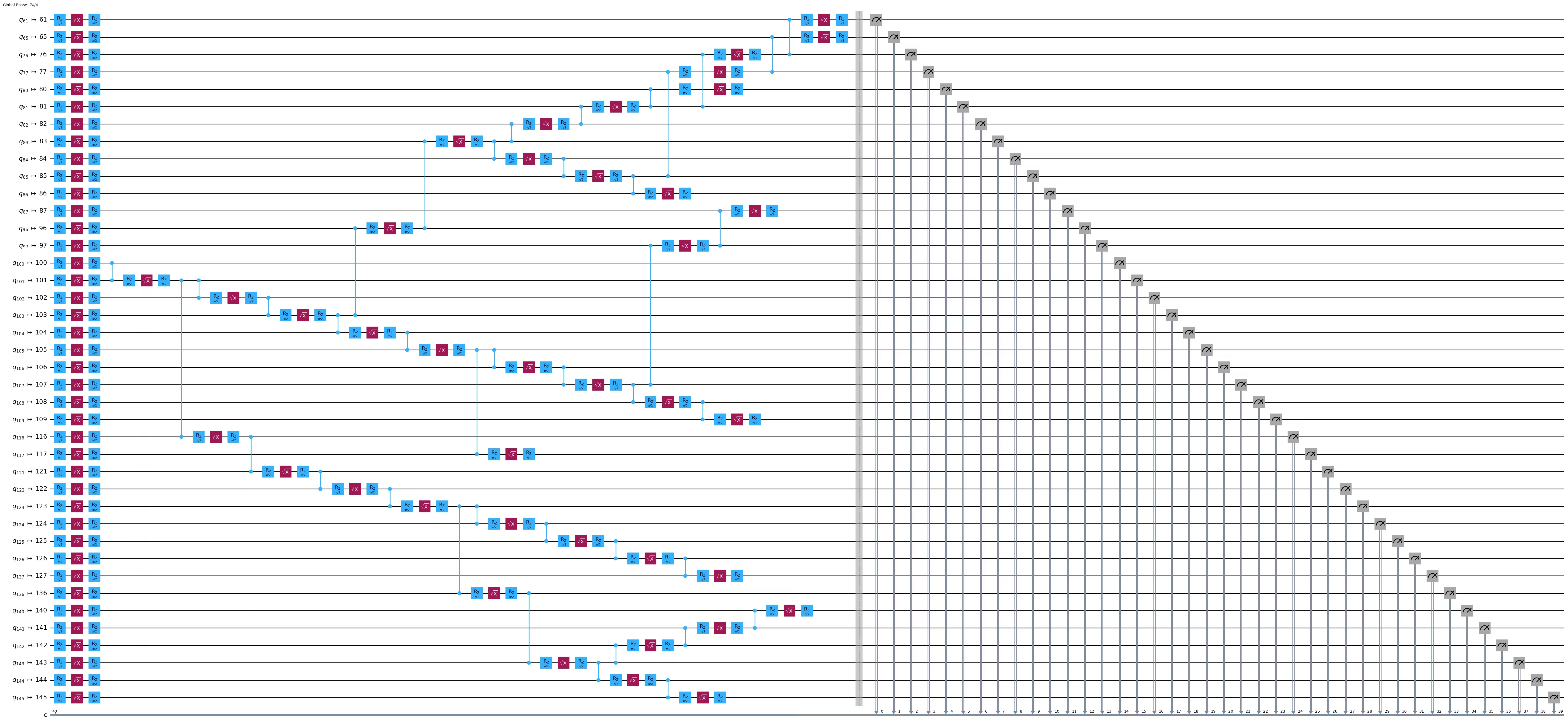
print("Depth:", ghz_h_transpiled.depth())
print(
    "Two-qubit Depth:",
    ghz_h_transpiled.depth(filter_function=lambda x: x.operation.num_qubits == 2),
)

Depth: 45
Two-qubit Depth: 13

opts = SamplerOptions()
opts.dynamical_decoupling.enable = True
opts.execution.rep_delay = 0.0005
opts.twirling.enable_gates = True

res = execute_ghz_fidelity(
    ghz_circuit=ghz_h,
    physical_qubits=best_qubits,
    backend=backend,
    sampler_options=opts,
)

job_s = service.job(res[0])  # Use your job id showed above.
job_e = service.job(res[1])
print(job_s.status(), job_e.status())

RUNNING RUNNING

# Check fidelity from job IDs
N = 40
res = check_ghz_fidelity_from_jobs(
    sampler_job=job_s,
    estimator_job=job_e,
    num_qubits=N,
)

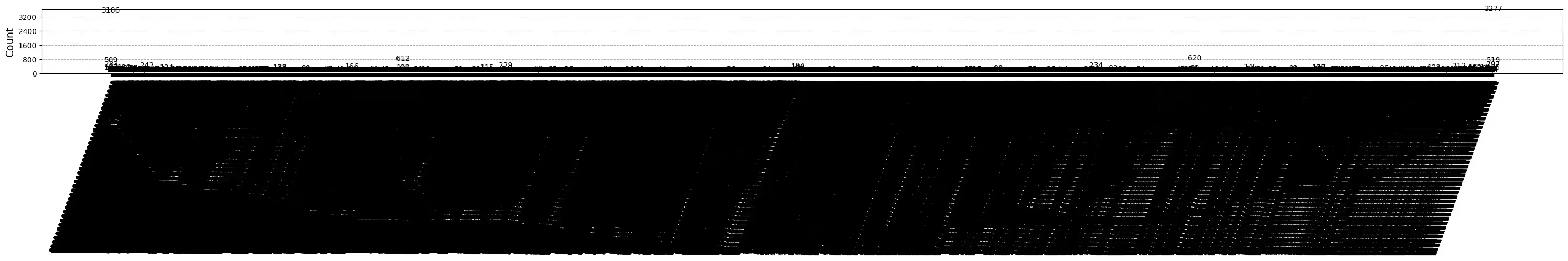
N=40: |00..0>: 3186, |11..1>: 3277, |3rd>: 620 (1111111011111111111111111111111111111111)
P(|00..0>)=0.07965, P(|11..1>)=0.081925
REM: Coherence (non-diagonal): 0.029987
GHZ fidelity = 0.095781 ± 0.002619
GME (genuinely multipartite entangled) test: Failed

# It will take some time
result = job_s.result()
plot_histogram(result[0].data.c.get_counts(), figsize=(30, 5))

¡Felicitaciones! Has completado tu introducción a la computación cuántica a escala utilitaria. ¡Ahora estás en posición de hacer contribuciones significativas en la búsqueda de la ventaja cuántica! Gracias por hacer de IBM Quantum® parte de tu viaje cuántico personal.

Encuesta posterior al curso

¡Felicitaciones por completar este curso! Por favor, tómate un momento para ayudarnos a mejorar nuestro contenido completando la siguiente encuesta breve. Tu opinión se utilizará para mejorar nuestra oferta de contenido y la experiencia de usuario. ¡Gracias!