Entradas y salidas de las primitivas

Package versions

El código de esta página fue desarrollado con los siguientes requisitos. Recomendamos usar estas versiones o versiones más recientes.

qiskit[all]~=2.4.0

Esta página ofrece una descripción general de las entradas y salidas de las primitivas de Qiskit. Con estas primitivas puedes usar una estructura de datos conocida como Primitive Unified Bloc (PUB) para definir cargas de trabajo vectorizadas de manera eficiente. Estos PUBs son la unidad fundamental de trabajo para la ejecución de cargas de trabajo. Se utilizan como entradas al método run() de las primitivas Sampler y Estimator, que ejecutan la carga de trabajo definida como un job. Luego, una vez que el job ha finalizado, los resultados se devuelven en un formato que depende de los PUBs utilizados y de cualquier opción especificada.

Descripción general de los PUBs

Al invocar el método run() de una primitiva, el argumento principal requerido es una list de una o más tuplas — una por cada circuito que ejecuta la primitiva. Cada una de estas tuplas se considera un PUB, y los elementos requeridos en cada tupla de la lista dependen de la primitiva utilizada. Los datos proporcionados a estas tuplas también pueden organizarse en distintas formas para aportar flexibilidad a una carga de trabajo mediante broadcasting — cuyas reglas se describen en una sección posterior.

PUB del Estimator

Para la primitiva Estimator, el formato del PUB debe contener como máximo cuatro valores:

• Un único QuantumCircuit, que puede contener uno o más objetos Parameter
• Una lista de uno o más observables que especifican los valores de expectación a estimar, organizados en un arreglo (por ejemplo, un único observable representado como un arreglo de 0 dimensiones, una lista de observables como un arreglo de 1 dimensión, etcétera). Los datos pueden estar en cualquiera de los formatos ObservablesArrayLike, como Pauli, SparsePauliOp, PauliList o str.
  nota

  Si tienes dos observables que conmutan en PUBs distintos pero con el mismo circuito, no se estimarán usando la misma medición. Cada PUB representa una base diferente de medición y, por lo tanto, se requieren mediciones separadas para cada PUB. Para garantizar que los observables que conmutan se estimen usando la misma medición, deben agruparse dentro del mismo PUB.

• Una colección de valores de parámetros para enlazar con el circuito. Esto puede especificarse como un único objeto tipo arreglo donde el último índice corresponde a los objetos Parameter del circuito, u omitirse (o de forma equivalente, establecerse como None) si el circuito no tiene objetos Parameter.
• (Opcionalmente) una precisión objetivo para los valores de expectación a estimar

PUB del Sampler

Para la primitiva Sampler, el formato de la tupla PUB contiene como máximo tres valores:

• Un único QuantumCircuit, que puede contener uno o más objetos Parameter Nota: Estos circuitos deben incluir instrucciones de medición para cada uno de los qubits a muestrear.
• Una colección de valores de parámetros para enlazar con el circuito $\theta_k$ (solo necesaria si se usan objetos Parameter que deben enlazarse en tiempo de ejecución)
• (Opcionalmente) un número de shots con el que medir el circuito

---

El siguiente código muestra un ejemplo de entradas vectorizadas a la primitiva Estimator.

# Added by doQumentation — required packages for this notebook
!pip install -q numpy qiskit

from qiskit.circuit import (
    Parameter,
    QuantumCircuit,
    ClassicalRegister,
    QuantumRegister,
)
from qiskit.transpiler import generate_preset_pass_manager
from qiskit.quantum_info import SparsePauliOp
from qiskit.primitives.containers import BitArray
from qiskit.primitives import StatevectorEstimator

import numpy as np

# Define a circuit with two parameters.
circuit = QuantumCircuit(2)
circuit.h(0)
circuit.cx(0, 1)
circuit.ry(Parameter("a"), 0)
circuit.rz(Parameter("b"), 0)
circuit.cx(0, 1)
circuit.h(0)

# Transpile the circuit without providing a backend
pm = generate_preset_pass_manager(optimization_level=1)
transpiled_circuit = pm.run(circuit)
layout = transpiled_circuit.layout

# Now define a sweep over parameter values, the last axis of dimension 2 is
# for the two parameters "a" and "b"
params = np.vstack(
    [
        np.linspace(-np.pi, np.pi, 10),
        np.linspace(-4 * np.pi, 4 * np.pi, 10),
    ]
).T

# Define three observables. The inner length-1 lists cause this array of
# observables to have shape (3, 1), rather than shape (3,) if they were
# omitted.
observables = [
    [SparsePauliOp(["XX", "IY"], [0.5, 0.5])],
    [SparsePauliOp("XX")],
    [SparsePauliOp("IY")],
]
# Apply the same layout as the transpiled circuit.
observables = [
    [observable.apply_layout(layout) for observable in observable_set]
    for observable_set in observables
]

# Estimate the expectation value for all 300 combinations of observables
# and parameter values, where the pub result will have shape (3, 100).
#
# This shape is due to our array of parameter bindings having shape
# (100, 2), combined with our array of observables having shape (3, 1).
estimator = StatevectorEstimator()
estimator_pub = (transpiled_circuit, observables, params)

# Run the transpiled circuit
# using the set of parameters and observables.

job = estimator.run([estimator_pub])
result = job.result()

Reglas de broadcasting

Los PUBs agregan elementos de múltiples arreglos (observables y valores de parámetros) siguiendo las mismas reglas de broadcasting que NumPy. Esta sección resume brevemente esas reglas. Para una explicación detallada, consulta la documentación de reglas de broadcasting de NumPy.

Reglas:

• Los arreglos de entrada no necesitan tener el mismo número de dimensiones.
  • El arreglo resultante tendrá el mismo número de dimensiones que el arreglo de entrada con mayor dimensión.
  • El tamaño de cada dimensión es el tamaño más grande de la dimensión correspondiente.
  • Se asume que las dimensiones faltantes tienen tamaño uno.
• Las comparaciones de forma comienzan por la dimensión más a la derecha y continúan hacia la izquierda.
• Dos dimensiones son compatibles si sus tamaños son iguales o si uno de ellos es 1.

Ejemplos de pares de arreglos que hacen broadcasting:

A1     (1d array):      1
A2     (2d array):  3 x 5
Result (2d array):  3 x 5

A1     (3d array):  11 x 2 x 7
A2     (3d array):  11 x 1 x 7
Result (3d array):  11 x 2 x 7

Ejemplos de pares de arreglos que no hacen broadcasting:

A1     (1d array):  5
A2     (1d array):  3

A1     (2d array):      2 x 1
A2     (3d array):  6 x 5 x 4 # This would work if the middle dimension were 2, but it is 5.

Estimator devuelve una estimación del valor de expectación por cada elemento de la forma resultante del broadcasting.

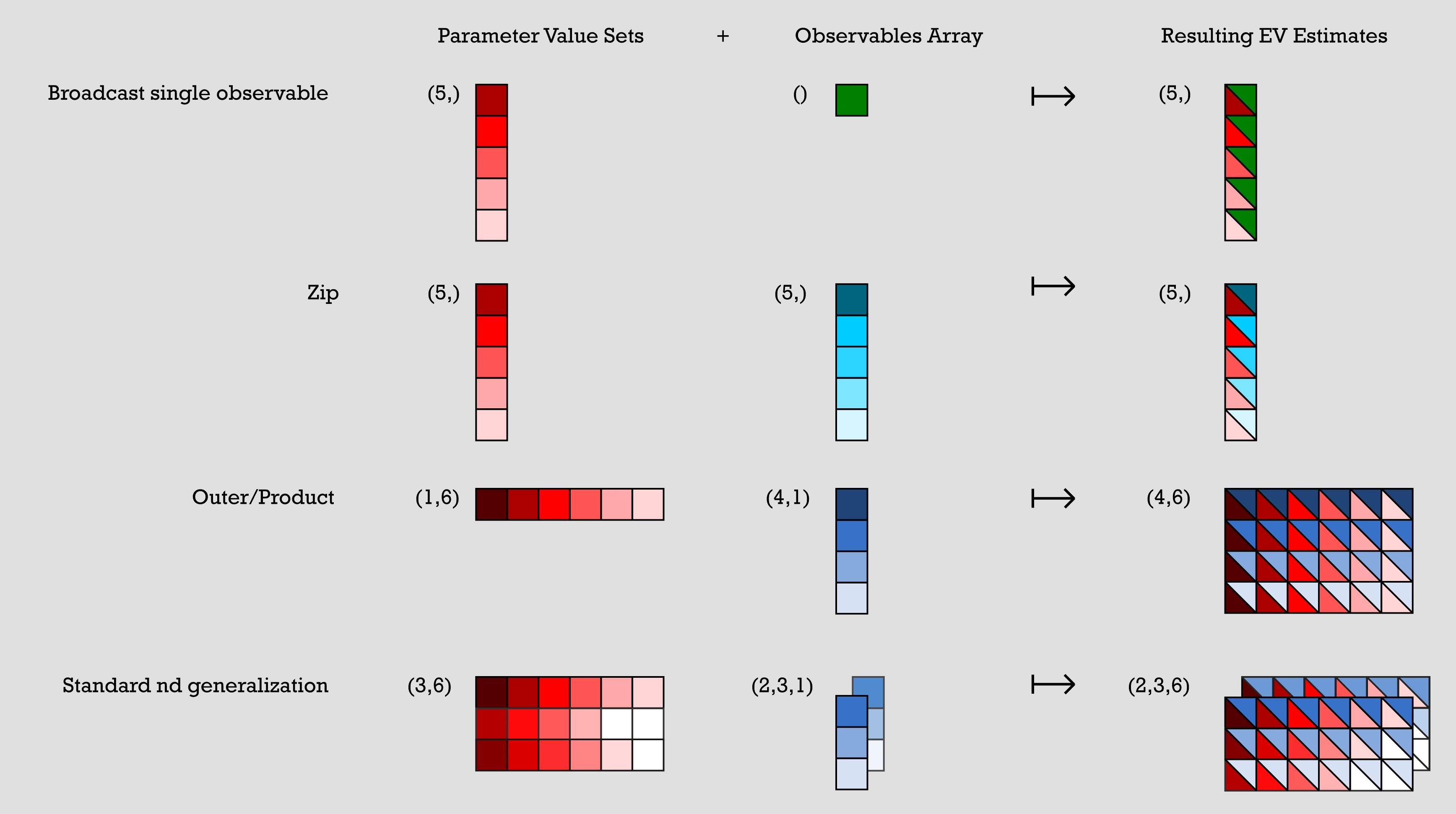
A continuación se presentan algunos ejemplos de patrones comunes expresados en términos de broadcasting de arreglos. Su representación visual correspondiente se muestra en la figura siguiente:

Los conjuntos de valores de parámetros se representan como arreglos de n x m, y los arreglos de observables se representan como uno o más arreglos de una sola columna. Para cada ejemplo en el código anterior, los conjuntos de valores de parámetros se combinan con su arreglo de observables para crear las estimaciones de valores de expectación resultantes.

• Ejemplo 1: (broadcast de un único observable) tiene un conjunto de valores de parámetros que es un arreglo de 5x1 y un arreglo de observables de 1x1. El único elemento del arreglo de observables se combina con cada elemento del conjunto de valores de parámetros para crear un único arreglo de 5x1 donde cada elemento es una combinación del elemento original en el conjunto de valores de parámetros con el elemento del arreglo de observables.

• Ejemplo 2: (zip) tiene un conjunto de valores de parámetros de 5x1 y un arreglo de observables de 5x1. La salida es un arreglo de 5x1 donde cada elemento es una combinación del n-ésimo elemento del conjunto de valores de parámetros con el n-ésimo elemento del arreglo de observables.

• Ejemplo 3: (producto exterior) tiene un conjunto de valores de parámetros de 1x6 y un arreglo de observables de 4x1. Su combinación produce un arreglo de 4x6 que se crea combinando cada elemento del conjunto de valores de parámetros con cada elemento del arreglo de observables, por lo que cada valor de parámetro se convierte en una columna completa en la salida.

• Ejemplo 4: (generalización nd estándar) tiene un arreglo de valores de parámetros de 3x6 y dos arreglos de observables de 3x1. Estos se combinan para crear dos arreglos de salida de 3x6 de manera similar al ejemplo anterior.

# Broadcast single observable
parameter_values = np.random.uniform(size=(5,))  # shape (5,)
observables = SparsePauliOp("ZZZ")  # shape ()
# >> pub result has shape (5,)

# Zip
parameter_values = np.random.uniform(size=(5,))  # shape (5,)
observables = [
    SparsePauliOp(pauli) for pauli in ["III", "XXX", "YYY", "ZZZ", "XYZ"]
]  # shape (5,)
# >> pub result has shape (5,)

# Outer/Product
parameter_values = np.random.uniform(size=(1, 6))  # shape (1, 6)
observables = [
    [SparsePauliOp(pauli)] for pauli in ["III", "XXX", "YYY", "ZZZ"]
]  # shape (4, 1)
# >> pub result has shape (4, 6)

# Standard nd generalization
parameter_values = np.random.uniform(size=(3, 6))  # shape (3, 6)
observables = [
    [
        [SparsePauliOp(["XII"])],
        [SparsePauliOp(["IXI"])],
        [SparsePauliOp(["IIX"])],
    ],
    [
        [SparsePauliOp(["ZII"])],
        [SparsePauliOp(["IZI"])],
        [SparsePauliOp(["IIZ"])],
    ],
]  # shape (2, 3, 1)
# >> pub result has shape (2, 3, 6)

a = SparsePauliOp("Z") # shape ()
b = SparsePauliOp("IIIIZXYIZ") # shape ()
c = SparsePauliOp.from_list(["XX", "XY", "IZ"]) # shape ()

SparsePauliOp

Cada SparsePauliOp cuenta como un único elemento en este contexto, independientemente de la cantidad de Paulis que contenga el SparsePauliOp. Por lo tanto, para los fines de estas reglas de broadcasting, todos los elementos siguientes tienen la misma forma:

list1 = SparsePauliOp.from_list(["XX", "XY", "IZ"]) # shape ()
list2 = [SparsePauliOp("XX"), SparsePauliOp("XY"), SparsePauliOp("IZ")] # shape (3, )

Descripción general de las salidas de las primitivas

Una vez que uno o más PUBs se envían a un QPU para su ejecución y el job finaliza con éxito, los datos se devuelven como un objeto contenedor PrimitiveResult. El PrimitiveResult contiene una lista iterable de objetos PubResult que contienen los resultados de ejecución de cada PUB. Por ejemplo, un job enviado con 20 PUBs devolverá un objeto PrimitiveResult que contiene una lista de 20 PubResults, uno por cada PUB.

Cada uno de estos objetos PubResult posee tanto un atributo data como un atributo metadata opcional. El atributo data es un DataBin personalizado que contiene las estimaciones de valores de expectación en el caso del Estimator, o muestras de la salida del circuito en el caso del Sampler.

El atributo data también puede incluir otra información específica de la implementación, como desviaciones estándar. El atributo metadata puede contener información adicional específica de la implementación sobre la ejecución del PUB asociado.

A continuación se presenta un esquema visual de la estructura de datos de PrimitiveResult:

Estimator output

└── PrimitiveResult
    ├── PubResult[0]
    │   ├── metadata
    │   └── data  ## In the form of a DataBin object,
    |       |     ## which includes data such as the following:
    │       ├── evs
    │       │   └── List of estimated expectation values in the shape
    |       |         specified by the first pub
    │       └── stds
    │           └── List of calculated standard deviations in the
    |                 same shape as above
    ├── PubResult[1]
    |   ├── metadata
    |   └── data  ## In the form of a DataBin object,
    |       |     ## which includes data such as the following:
    |       ├── evs
    |       │   └── List of estimated expectation values in the shape
    |       |        specified by the second pub
    |       └── stds
    |           └── List of calculated standard deviations in the
    |                same shape as above
    ├── ...
    ├── ...
    └── ...

nota

Lo anterior es un ejemplo de los datos que pueden devolverse. Los datos reales devueltos dependen de la implementación.

Sampler output

└── PrimitiveResult
    ├── PubResult[0]
    │   ├── metadata
    │   └── data  ## In the form of a DataBin object
    │       ├── NAME_OF_CLASSICAL_REGISTER
    │       │   └── BitArray of count data for first PUB (default is 'meas')
    |       |
    │       └── NAME_OF_ANOTHER_CLASSICAL_REGISTER
    │           └── BitArray of count data (exists only if more than one
    |                 ClassicalRegister was specified in the circuit)
    ├── PubResult[1]
    |   ├── metadata
    |   └── data  ## In the form of a DataBin object
    |       └── NAME_OF_CLASSICAL_REGISTER
    |           └── BitArray of count data for second PUB
    ├── ...
    ├── ...
    └── ...

Salida del Estimator

Como se indicó anteriormente, los datos devueltos en el PubResult para la primitiva Estimator dependen de la implementación. Por ejemplo, puede contener un arreglo de valores de expectación (PubResult.data.evs) y las desviaciones estándar asociadas (PubResult.data.stds).

El siguiente fragmento de código describe el formato de PrimitiveResult (y el PubResult asociado) para el job creado anteriormente.

print(
    f"The result of the submitted job had {len(result)} PUB and has a value:\n {result}\n"
)
print(
    f"The associated PubResult of this job has the following data bins:\n {result[0].data}\n"
)
print(f"And this DataBin has attributes: {result[0].data.keys()}")
print(
    "Recall that this shape is due to our array of parameter binding sets having shape (100, 2) -- where 2 is the\n\
         number of parameters in the circuit -- combined with our array of observables having shape (3, 1). \n"
)
print(
    f"The expectation values measured from this PUB are: \n{result[0].data.evs}"
)

The result of the submitted job had 1 PUB and has a value:
 PrimitiveResult([PubResult(data=DataBin(evs=np.ndarray(<shape=(3, 10), dtype=float64>), stds=np.ndarray(<shape=(3, 10), dtype=float64>), shape=(3, 10)), metadata={'target_precision': 0.0, 'circuit_metadata': {}})], metadata={'version': 2})

The associated PubResult of this job has the following data bins:
 DataBin(evs=np.ndarray(<shape=(3, 10), dtype=float64>), stds=np.ndarray(<shape=(3, 10), dtype=float64>), shape=(3, 10))

And this DataBin has attributes: dict_keys(['evs', 'stds'])
Recall that this shape is due to our array of parameter binding sets having shape (100, 2) -- where 2 is the
         number of parameters in the circuit -- combined with our array of observables having shape (3, 1). 

The expectation values measured from this PUB are: 
[[ 3.06161700e-16  4.52395120e-01  4.36594428e-01  2.16506351e-01
   6.33718361e-01 -6.33718361e-01 -2.16506351e-01 -4.36594428e-01
  -4.52395120e-01 -3.06161700e-16]
 [ 1.22464680e-16  6.42787610e-01  9.84807753e-01  8.66025404e-01
   3.42020143e-01 -3.42020143e-01 -8.66025404e-01 -9.84807753e-01
  -6.42787610e-01 -1.22464680e-16]
 [ 4.89858720e-16  2.62002630e-01 -1.11618897e-01 -4.33012702e-01
   9.25416578e-01 -9.25416578e-01  4.33012702e-01  1.11618897e-01
  -2.62002630e-01 -4.89858720e-16]]

Salida del Sampler

Cuando un job de Sampler se completa con éxito, el objeto PrimitiveResult devuelto contiene una lista de SamplerPubResult, uno por PUB. Los data bins de estos objetos SamplerPubResult son objetos similares a diccionarios que contienen un BitArray por cada ClassicalRegister del circuito.

La clase BitArray es un contenedor para datos de shots ordenados. En más detalle, almacena las cadenas de bits muestreadas como bytes dentro de un array bidimensional. El eje más a la izquierda de este array recorre los shots en orden, mientras que el eje más a la derecha recorre los bytes.

Como primer ejemplo, veamos el siguiente circuito de diez qubits:

from qiskit.primitives import StatevectorSampler

# generate a ten-qubit GHZ circuit
circuit = QuantumCircuit(10)
circuit.h(0)
circuit.cx(range(0, 9), range(1, 10))

# append measurements with the `measure_all` method
circuit.measure_all()

# transpile the circuit
transpiled_circuit = pm.run(circuit)

sampler = StatevectorSampler()

# run the Sampler job and retrieve the results

job = sampler.run([transpiled_circuit])
result = job.result()

# the data bin contains one BitArray
data = result[0].data
print(f"Databin: {data}\n")

# to access the BitArray, use the key "meas", which is the default name of
# the classical register when this is added by the `measure_all` method
array = data.meas
print(f"BitArray: {array}\n")
print(f"The shape of register `meas` is {data.meas.array.shape}.\n")
print(f"The bytes in register `alpha`, shot by shot:\n{data.meas.array}\n")

Databin: DataBin(meas=BitArray(<shape=(), num_shots=1024, num_bits=10>))

BitArray: BitArray(<shape=(), num_shots=1024, num_bits=10>)

The shape of register `meas` is (1024, 2).

The bytes in register `alpha`, shot by shot:
[[  0   0]
 [  3 255]
 [  0   0]
 ...
 [  3 255]
 [  3 255]
 [  3 255]]

# optionally, convert away from the native BitArray format to a dictionary format
counts = data.meas.get_counts()
print(f"Counts: {counts}")

Counts: {'0000000000': 492, '1111111111': 532}

A veces puede ser conveniente convertir el formato de bytes del BitArray a cadenas de bits. El método get_count devuelve un diccionario que mapea cadenas de bits al número de veces que ocurrieron.

# generate a ten-qubit GHZ circuit with two classical registers
circuit = QuantumCircuit(
    qreg := QuantumRegister(10),
    alpha := ClassicalRegister(1, "alpha"),
    beta := ClassicalRegister(9, "beta"),
)
circuit.h(0)
circuit.cx(range(0, 9), range(1, 10))

# append measurements with the `measure_all` method
circuit.measure([0], alpha)
circuit.measure(range(1, 10), beta)

# transpile the circuit
transpiled_circuit = pm.run(circuit)

# run the Sampler job and retrieve the results

job = sampler.run([transpiled_circuit])
result = job.result()

# the data bin contains two BitArrays, one per register, and can be accessed
# as attributes using the registers' names
data = result[0].data
print(f"BitArray for register 'alpha': {data.alpha}")
print(f"BitArray for register 'beta': {data.beta}")

Cuando un circuito contiene más de un registro clásico, los resultados se almacenan en objetos BitArray distintos. El siguiente ejemplo modifica el fragmento anterior dividiendo el registro clásico en dos registros separados:

BitArray for register 'alpha': BitArray(<shape=(), num_shots=1024, num_bits=1>)
BitArray for register 'beta': BitArray(<shape=(), num_shots=1024, num_bits=9>)

print(f"The shape of register `alpha` is {data.alpha.array.shape}.")
print(f"The bytes in register `alpha`, shot by shot:\n{data.alpha.array}\n")

print(f"The shape of register `beta` is {data.beta.array.shape}.")
print(f"The bytes in register `beta`, shot by shot:\n{data.beta.array}\n")

# post-select the bitstrings of `beta` based on having sampled "1" in `alpha`
mask = data.alpha.array == "0b1"
ps_beta = data.beta[mask[:, 0]]
print(f"The shape of `beta` after post-selection is {ps_beta.array.shape}.")
print(f"The bytes in `beta` after post-selection:\n{ps_beta.array}")

# get a slice of `beta` to retrieve the first three bits
beta_sl_bits = data.beta.slice_bits([0, 1, 2])
print(
    f"The shape of `beta` after bit-wise slicing is {beta_sl_bits.array.shape}."
)
print(f"The bytes in `beta` after bit-wise slicing:\n{beta_sl_bits.array}\n")

# get a slice of `beta` to retrieve the bytes of the first five shots
beta_sl_shots = data.beta.slice_shots([0, 1, 2, 3, 4])
print(
    f"The shape of `beta` after shot-wise slicing is {beta_sl_shots.array.shape}."
)
print(
    f"The bytes in `beta` after shot-wise slicing:\n{beta_sl_shots.array}\n"
)

# calculate the expectation value of diagonal operators on `beta`
ops = [SparsePauliOp("ZZZZZZZZZ"), SparsePauliOp("IIIIIIIIZ")]
exp_vals = data.beta.expectation_values(ops)
for o, e in zip(ops, exp_vals):
    print(f"Exp. val. for observable `{o}` is: {e}")

# concatenate the bitstrings in `alpha` and `beta` to "merge" the results of the two
# registers
merged_results = BitArray.concatenate_bits([data.alpha, data.beta])
print(f"\nThe shape of the merged results is {merged_results.array.shape}.")
print(f"The bytes of the merged results:\n{merged_results.array}\n")

Aprovechando los objetos BitArray para un post-procesamiento eficiente

Dado que los arrays generalmente ofrecen mejor rendimiento en comparación con los diccionarios, es recomendable realizar cualquier post-procesamiento directamente sobre los objetos BitArray en lugar de hacerlo sobre diccionarios de conteos. La clase BitArray ofrece una variedad de métodos para realizar algunas operaciones comunes de post-procesamiento:

The shape of register `alpha` is (1024, 1).
The bytes in register `alpha`, shot by shot:
[[1]
 [1]
 [1]
 ...
 [0]
 [0]
 [1]]

The shape of register `beta` is (1024, 2).
The bytes in register `beta`, shot by shot:
[[  1 255]
 [  1 255]
 [  1 255]
 ...
 [  0   0]
 [  0   0]
 [  1 255]]

The shape of `beta` after post-selection is (0, 2).
The bytes in `beta` after post-selection:
[]
The shape of `beta` after bit-wise slicing is (1024, 1).
The bytes in `beta` after bit-wise slicing:
[[7]
 [7]
 [7]
 ...
 [0]
 [0]
 [7]]

The shape of `beta` after shot-wise slicing is (5, 2).
The bytes in `beta` after shot-wise slicing:
[[  1 255]
 [  1 255]
 [  1 255]
 [  1 255]
 [  1 255]]

Exp. val. for observable `SparsePauliOp(['ZZZZZZZZZ'],
              coeffs=[1.+0.j])` is: -0.017578125
Exp. val. for observable `SparsePauliOp(['IIIIIIIIZ'],
              coeffs=[1.+0.j])` is: -0.017578125

The shape of the merged results is (1024, 2).
The bytes of the merged results:
[[  3 255]
 [  3 255]
 [  3 255]
 ...
 [  0   0]
 [  0   0]
 [  3 255]]

Metadatos de los resultados

Además de los resultados de ejecución, los objetos PrimitiveResult y PubResult contienen un atributo de metadatos opcional sobre el job enviado. Los metadatos devueltos (si los hay) son específicos de la implementación.

# Print out the results metadata
print("The metadata of the PrimitiveResult is:")
for key, val in result.metadata.items():
    print(f"'{key}' : {val},")

print("\nThe metadata of the PubResult result is:")
for key, val in result[0].metadata.items():
    print(f"'{key}' : {val},")

The metadata of the PrimitiveResult is:
'version' : 2,

The metadata of the PubResult result is:
'shots' : 1024,
'circuit_metadata' : {},

Próximos pasos

Recomendaciones

• Revisa la API de las primitivas de Qiskit.
• Revisa la API de las primitivas de Qiskit Aer.
• Obtén más información sobre las primitivas de Qiskit Runtime.
• Revisa la API del Estimator de Qiskit Runtime.
• Revisa la API del Sampler de Qiskit Runtime.